Furthest Water

An analysis showing how to find the place in the US furthest from water.

Finding the Location Furthest from Water in the Conterminous United States

The idea for this post came a few months back when I received an email that started, “I am a writer and teacher and am reaching out to you with a question related to a piece I would like to write about the place in the United States that is furthest from a natural body of surface water. My question is, in short, might you know where this theoretical place is located?”

As someone who works on the National Water Census and National hydrography data, this question piqued my interest. I also had an idea of one way to answer the question that would use some tools and techniques I’ve recently been developing in R. What follows is just that, one way that this question might be answered. The code I used to find the solution is presented in detail after the solution to the question.

The solution graphics shown below were generated with the following code: The furthest_water.R script can be found here.

source("furthest_water.R")
furthest_water(scenario = "waterbodies")

furthest_water(scenario = c("waterbodies", "filter_monthly_flow"))

furthest_water(scenario = c("waterbodies", "remove_intermittent", "filter_monthly_flow"))

Method

To answer the question, “where is the furthest place from a natural body of water?”, I first had to decide where all the places I might want to check are. To do this, I first built a search box around the southwestern US to limit the data volume I had to process. I then created a grid of points 5km apart within the search box and the US coastline. This set of points, pictured below, will stand in for all the places we might want to look. Note that there are actually about 150k points on this image, but they draw as one area because their symbols overlap.

With all possible places defined, I needed all the water bodies. The National Hydrography Dataset contains data used to map rivers and lakes across the country. As a bonus, there is a dataset known as the “NHDPlus v2.1 National Seamless” that is available as a single geospatial database for the whole conterminous US. See this EPA page for lots of helpful documentation and data downloads. The NHDPlus contains a few million river segments and almost a half million water bodies mapped at 1:100,000-scale. The NHDPlus also has some useful attributes that categorize waterbodies as ephemeral (sometimes dry) or perennial (always wet) and modeled estimates of mean flow by month of the year for rivers. Geospatial data representing rivers and bodies of water like lakes along with the attributes about how likely they are to be wet is just what I needed. The maps below show how dense the rivers and water bodies in the NHDPlus are.

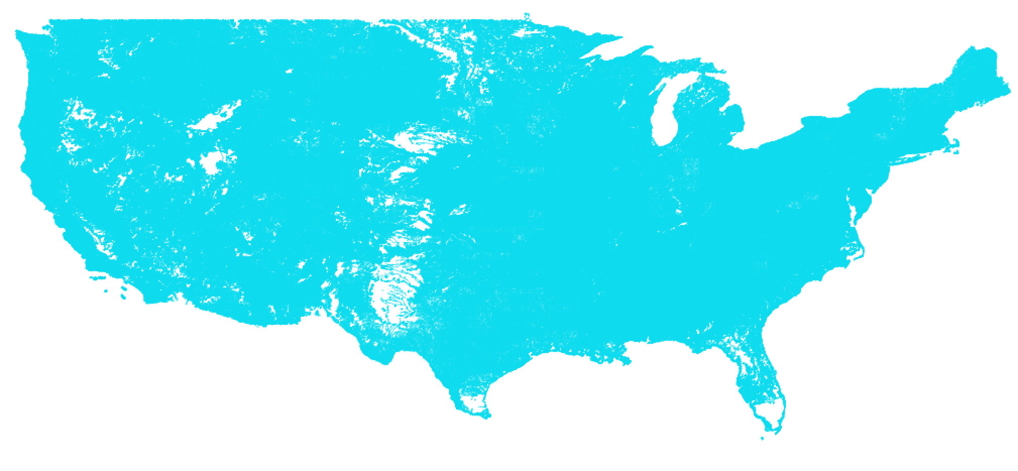
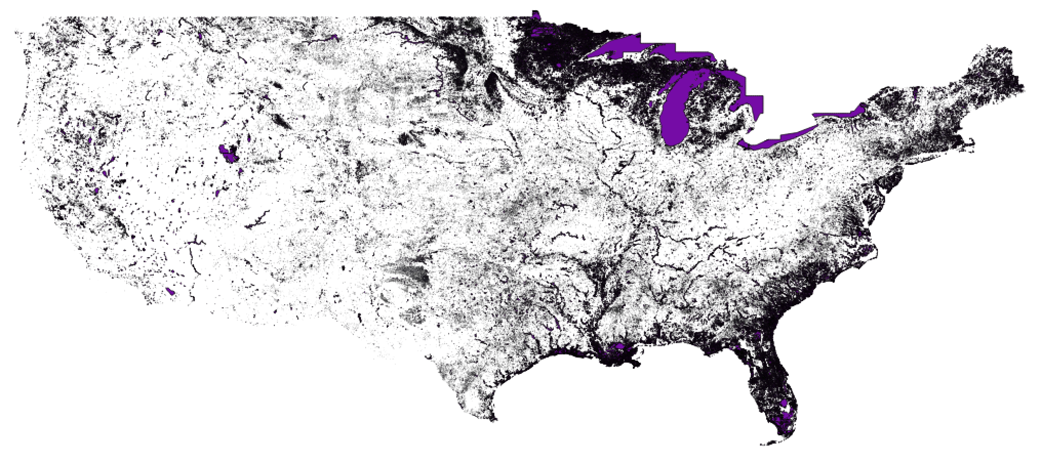
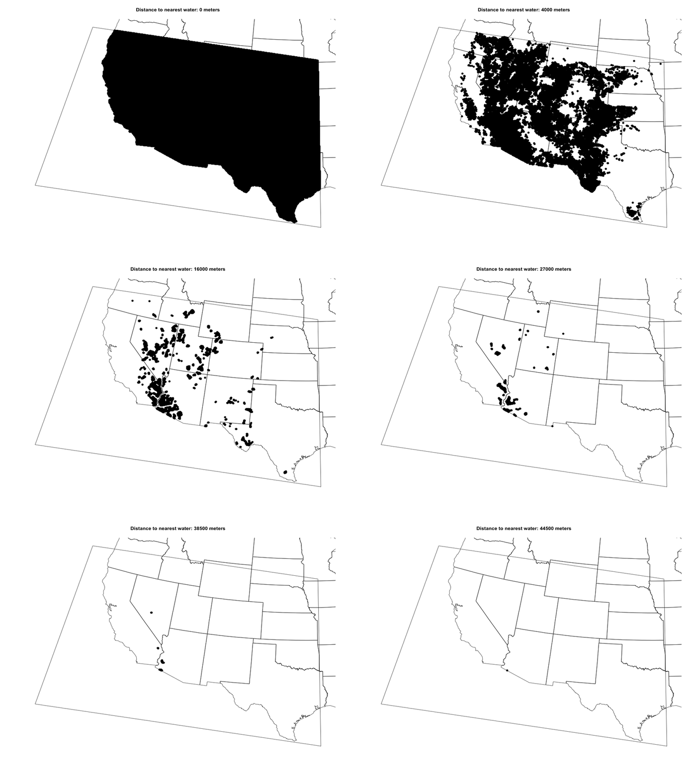
The algorithm I used to figure out which of the search locations is furthest from water uses a nearest neighbor search implemented in an R package called RANN which allowed me to find which points are within a given distance of a flowline or water body. By starting with a small distance and incrementing to larger and larger distances, removing locations as I went, I was able to narrow down to one point that was further than any other from all the water bodies. The marvel of this technique is that it’s not just 150k points and a few million rivers and lakes. To make it work, I converted the lines and polygons that represent rivers and water bodies to more than 30 million individual points that make up all the geometry!

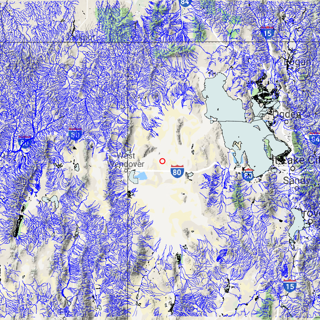
In each of the three scenarios below, there are two graphics. The first, is a simple visual showing where the location is relative to rivers and water bodies that are in the vicinity. The second is an animated graphic showing each step of the nearest neighbor search as the search radius increases incrementally.

Furthest from where there might be water

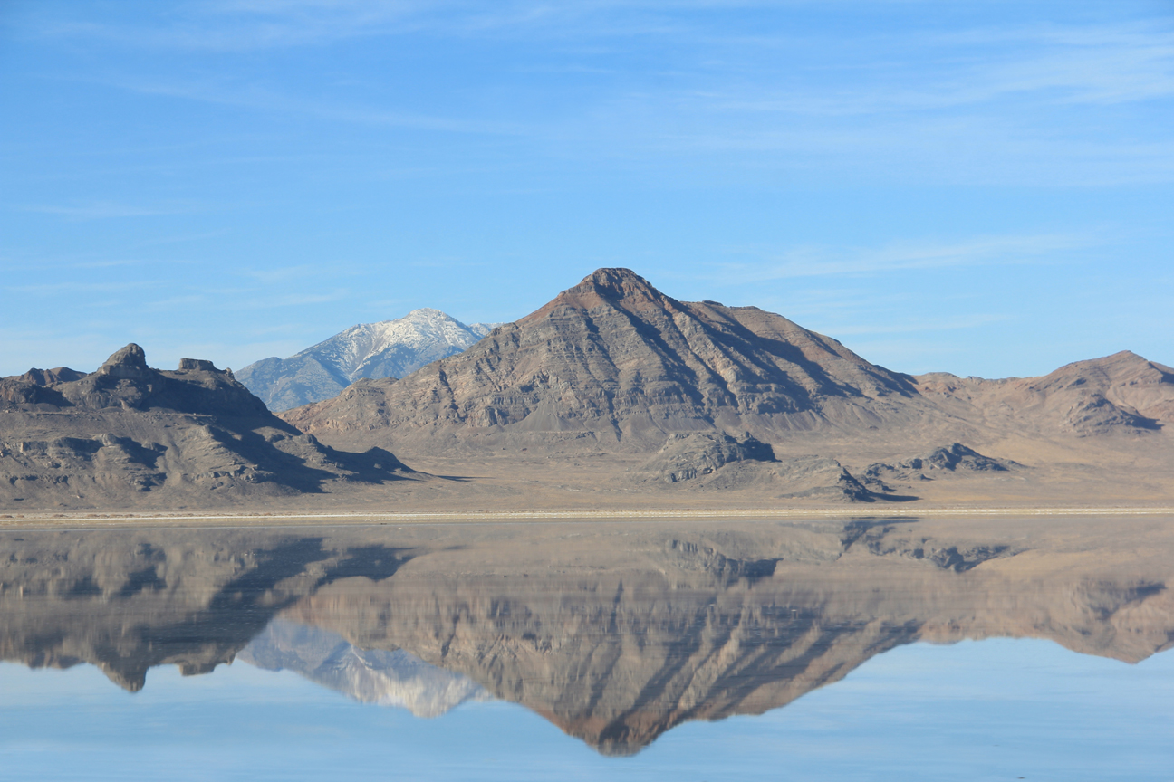
In the first scenario, I included everything in the NHDPlus that might be a water body. This includes lakes and rivers that are categorized as ephemeral and rivers with attributes that show they are usually dry one or more months a year. As you can see below, the location is in the Bonneville salt flats. The irony is that, while not categorized as a water body in the NHD, this picture taken from I-80 shows that the salt flats do get filled with water periodically!

By Ricraider - Own work, CC BY-SA 3.0, Link

Furthest from modeled water

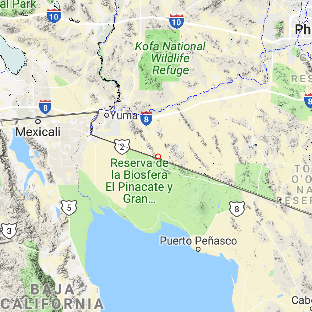
The place we say is the furthest from water shouldn’t be a dry lake bed, should it? Let’s look at another scenario. In this one, I used the monthly average flow estimates from the NHDPlus. These estimates are calculated using the “Enhanced Runoff Method” or EROM. You can find documentation about the method here. The EROM estimates are available for each month of the year, providing a normal monthly-mean flow estimate for the period of the analysis (1971 to 2000). For this scenario, I removed any flowline that had a monthly-mean flow estimate of zero for any month. As can be seen below, I came up with a location almost on the US-Mexico border in the desert in far south west Arizona.

This is a place I would believe is actually the furthest from a natural body of water but I noticed that there were some small waterbodies in the desert that almost certainly dry out in the summer.

Explore this place in google maps

Furthest from modeled and non-ephemeral water

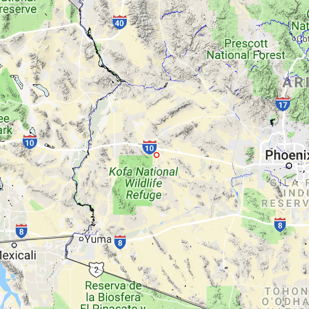
For the third scenario, I used the same mean-monthly flow method to remove rivers that probably dry out for a month or more a year and I removed flowlines and water bodies that were categorized as ephemeral. This removed many water body polygons in the desert that are only wet part of the year. As can be seen below, now we are in the Sonoran desert west of Phoenix, AZ. By the looks of things, this really may be the furthest from a natural body of surface water in the US (over 72km/45mi) – especially after a long period with no rain.

Explore this place in google maps

As the variety of results given different inputs shows, this question doesn’t necessarily have one answer. It depends what we assume a body of water is and how often that body of water needs to be wet. The factors at play that determine if a river or water body is wet are diverse and highly interrelated. Ranging from the obvious, like how much it’s rained recently, to less obvious, like how much groundwater is flowing into or out of a river. Ecosystems have a role to play too. In desert environments, some plants depend on groundwater which can actually draw down groundwater around rivers, reducing flows or even causing surface flow to cease even though groundwater may continue to be available just under the surface. This is just a brief discussion of the complexities of the natural water cycle and the natural features that arise from it. For more, the USGS Water Science School has a wealth of information and all USGS publications and data are free and available for everyone.

Code Explanation

The three scenarios above were run using a function that executes the code described below. There is a mix of comments and summary text written outside the code. To execute this, you will need to install the required packages and download the NHDPlus National Seamless Database and a state boundaries layer available here. These two datasets are referenced in the code.

Load Packages and Data

In this first step, I load all the packages and data I need.

Packages include:

• sf
• dplyr
• RANN
• nhdplusTools
• units
• stringr
• gifski
• ggmap

Note that sf and dplyr do the vast majority of the work and they are loaded with a library() command. All other packages are accessed using the package::function() syntax

Variables created here are:

• flowlines: NHDPlus flowlines with lots of attributes. Loaded with nhdplusTools as a helper.
• water_bodies: NHDPlus waterbodies loaded directly from the National Seamless using sf read_sf().
• min_monthlies: Minimum of the twelve monthly flow estimates for each flowline. Calculated by applying the min function to all the monthly flow collumns from the flowlines attributes.
• remove_fcodes: NHDPlus feature codes that should be removed.
• crs: A coordinate reference system to perform the analysis in.
• states: A set of US state boundaries loaded from shapefile with sf.
• bbox: A bounding box to limit the analysis to less than the whole country. Created in the sf bbox format then converted in an sfc geometry.

library(sf)
library(dplyr)
# to install nhdplusTools
# devtools::install_github("dblodgett-usgs/nhdplusTools")
# First we will use a nhdplusTools to load up the national seamless geodatabase.
nhdplusTools::nhdplus_path("nhdplus_data/NHDPlusV21_National_Seamless.gdb")
staged_data <- nhdplusTools::stage_national_data(include = "flowline",
                                                 output_path = "nhdplus_data/")
flowlines <- readRDS(staged_data$flowline)

# Now lets read in the waterbodies directly from the national seamless database.
if("waterbodies" %in% scenario) {
  water_bodies <- read_sf(nhdplus_path(), "NHDWaterbody")
}

if("filter_monthly_flow" %in% scenario) {
  monthlies <- which(grepl("QA_[0-1][0-9]", names(flowlines)))
  min_monthlies <- apply(st_set_geometry(flowlines, NULL)[monthlies], 1, min)
}

if("remove_intermittent" %in% scenario) {
  fcodes <- read_sf(nhdplus_path(), "NHDFCode")
  remove_fcodes <- fcodes[which(fcodes$Hydrograph == "Intermittent"), ]
}

# http://spatialreference.org/ref/sr-org/epsg-5070/
crs <- st_crs(5070)

# See: https://www.arcgis.com/home/item.html?id=b07a9393ecbd430795a6f6218443dccc for this file
states <- read_sf("states_21basic/states.shp")

# http://bboxfinder.com/#25.284438,-127.265625,43.707594,-94.438477
bbox <- c(-127.265625,25.284438,-94.438477,43.7075949)
names(bbox) <- c("xmin", "ymin", "xmax", "ymax")
class(bbox) <- "bbox"
bbox <- st_as_sfc(bbox)
st_crs(bbox) <- 4326

Transform and Filter

In this next step, I transform all the data into a consistent coordinate reference system and get everything filtered. This is all the data I want to use for the actual nearest neighbor search. Processing includes:

• states: Transform to analysis coordinate system and remove small islands. - flowlines and water_bodies: Filter out flowlines with min monthly flow of 0 and feature codes indicating intermittent. Transform to analysis coordinate system and intersect with analysis bounds and simplify geometry to remove un-needed data and precision.

At this point, I save the input flowlines and waterbodies to disk for use later because the process is destructive and I need to be careful how much system memory I’m using.

bbox <- st_transform(bbox, crs)

states <- states %>%
  st_transform(crs) %>%
  st_cast("POLYGON") %>%
  mutate(AREA = st_area(.)) %>%
  filter(AREA > units::set_units(2500000000, "m^2")) %>%
  select(-AREA)

if("filter_monthly_flow" %in% scenario) {
  flowlines <- flowlines[which(min_monthlies !=0 ), ]
}

if("remove_intermittent" %in% scenario) {
  flowlines <- flowlines[which(!flowlines$FCODE %in% remove_fcodes$FCode), ]
  if("waterbodies" %in% scenario) {
    water_bodies <- water_bodies[which(!water_bodies$FCODE %in% remove_fcodes$FCode), ]
  }
}

flowlines <- flowlines %>%
  st_transform(crs) %>%
  st_simplify(1000) %>%
  st_intersection(bbox)

if("waterbodies" %in% scenario) {
  water_bodies <-
    st_transform(water_bodies, crs) %>%
    st_buffer(0) %>%
    st_simplify(500) %>%
    st_intersection(bbox)
}

# Save some intermediate artifacts that we'll read back in later.
saveRDS(flowlines, "temp_flowlines.rds")
if("waterbodies" %in% scenario) saveRDS(water_bodies, "temp_water_bodies.rds")

Convert to coordinates

Now that I have all my data in the right coordinate system and have removed all the data that I don’t want, I can set up the data for the actual nearest neighbor search. This code converts the data to coordinate pairs with a set of identifiers for each feature and feature part. Some of this code is not used, but is included to demonstrate how identifiers work in what comes out of sf::st_coordinates. The “MULTILINESTRING” coordinates have columns X, Y, L1, and L2 where L1 is the part number and L2 is the overall feature. The “MULTIPOLYGON” coordinates have columns X, Y, L1, L2, and L3 where L1 is for the main ring or holes, L2 for each polygon, and L3 for the overall feature. In this case, I just extract the identifier for the overall feature and could have used that information to track back to the actual water body or flowline in particular that I end up with at the end.

if("waterbodies" %in% scenario) wb_COMID <- water_bodies$COMID
fl_COMID <- flowlines$COMID

# Now turn both flowlines and water_bodies into coordinate pairs only
flowlines <-
  st_cast(flowlines, "MULTILINESTRING") %>%
  st_coordinates()
if("waterbodies" %in% scenario) {
  water_bodies <-
    st_cast(water_bodies, "MULTIPOLYGON") %>%
    st_coordinates()
}

# Extract the identifier of features from the coordinates
flowlines <- flowlines[,c(1,2,4)] %>%
  data.frame() %>%
  rename(ID = L2)
if("waterbodies" %in% scenario) {
  water_bodies <- water_bodies[,c(1,2,5)] %>%
    data.frame() %>%
    rename(ID = L3)
}

# Switch the new ID column to the "COMID" values from the source data.
if("waterbodies" %in% scenario) {
  water_bodies[["COMID"]] <- wb_COMID[water_bodies[["ID"]]]
}
flowlines[["COMID"]] <- fl_COMID[flowlines[["ID"]]]

# Bind together into one huge set of coordinates.
if("waterbodies" %in% scenario) {
  coords <- rbind(water_bodies, flowlines) %>%
    select(-ID)
  rm(flowlines, water_bodies)
} else {
  coords <- flowlines %>%
    select(-ID)
  rm(flowlines)
}

Search Points

In this short step, I create my set of all points using the function expand.grid() and the extents of the bounding box I created above. Using the complete grid of locations, I convert it to as sf data.frame and remove all the points outside the analysis box and outside the states. I then convert the set of points inside the analysis area to a data.frame() of coordinates.

# Create a set of search locations
search_bbox <- st_bbox(bbox)
x <- seq(search_bbox$xmin, search_bbox$xmax, 5000)
y <- seq(search_bbox$ymin, search_bbox$ymax, 5000)
search <- expand.grid(x,y)

# Convert to sf and intersect with the state boundaries.
search <- st_as_sf(data.frame(search), coords = c("Var1", "Var2"), crs = crs) %>%
  st_intersection(states) %>%
  st_intersection(bbox) %>%
  st_coordinates() %>%
  data.frame()

Plot function

In order to create the animated gif, I needed to be able to create a similar plot over and over. So I created a function to do the job. This function creates an output file name, sets up a png, gets the data ready to plot, then plots a few layers using base R graphics and plot.sf.

# Function to plot results in a .png
plot_result <- function(search, radius, crs, bbox, states) {
  fname <- stringr::str_pad(paste0(as.character(radius), ".png"), 10, "left", "0")
  png(fname,
      width = 1000, height = 800)
  result <- st_as_sf(search, coords = c("X", "Y"), crs = crs)

  plot(bbox, main = paste("Distance to nearest water:", radius, "meters"))
  plot(states$geometry, add = TRUE)
  plot(result$geometry, pch = 19, add = TRUE)
  dev.off()
}

Run the nearest neighbor search

Finally, we are ready to run the analysis. To me, while loops are the forbidden fruit of software development, but sometimes you just don’t know how many times you need to run a loop! In this case, we run the RANN::nn2() function which returns the index of the matching nearest neighbor (nn.idx), if one is found. If no nearest neighbor is found in the search radius, it returns nn.idx of 0. So in every loop, I only keep matches where nn.idx == 0 returns true. I plot the filtered set to a png and increment the radius up for the next loop. The if/else block at the bottom of this step just slows down the rate of increase of the radius as we approach only one location left to avoid overshooting and missing the last one!

Once the while loop finishes, I pass the list of pngs created to gifski a great little package for creating animated gifs. Finally I printed out the lat/lon of the location found so I could go look at the location in google.

radius <- 0
num_left <- nrow(search)

while(num_left > 1) {
  num_left <- nrow(search)

  # This is where the magic happens.
  matched <- RANN::nn2(coords[,1:2],
                       search,
                       k = 1,
                       searchtype = "radius",
                       radius = radius) %>%
    data.frame()

  # This while loop is destructive. Only keep unmatched.
  search <- filter(search, matched$nn.idx == 0)

  plot_result(search, radius, crs, bbox, states)

  if(num_left > 50) {
    radius <- radius + 1000
  } else if (num_left > 3) {
    radius <- radius + 500
  } else {
    radius <- radius + 100
  }
}

rm(coords)

gifski::gifski(list.files(pattern = "*0.png"))

# Where in the world is the result?
result <- st_as_sf(search, coords = c("X", "Y"), crs = crs)
print(st_transform(result$geometry, 4326))

Plot the result location

Finally, I plot up the results at a local scale. Steps for this include:

• I want the original data I started with, so I just load it back from disk. - I set up an area for the plot by buffering around the result location by 150km and converting the result to a simple box. - Increasingly, I like using the web mercator projection for visualization because it’s familiar and compatible with web-map tiles. - I project all the data to my plotting projection and subset it and simplify the geometry to speed things up and not overwhelm plot() with data for the whole country. - I grab a background map from google with ggmap::getmap to be passed to the bgMap input of plot.sf(). - I plot each layer I want into a png. - Finally I delete the png files and temporary geometry I wrote to disk.

# Load geospatial data again.
flowlines <- readRDS("temp_flowlines.rds")
if("waterbodies" %in% scenario) water_bodies <- readRDS("temp_water_bodies.rds")

# Set up a plot area around our result.
plot_area <- st_buffer(result$geometry, 150000) %>%
  st_bbox() %>%
  st_as_sfc()
st_crs(plot_area) <- crs

# Use 3857 (web mercator) for visualization.
plot_proj <- 3857
plot_area <- st_transform(plot_area, plot_proj)

# Subset data to an area that satisfies plot_area.
data_area <- st_bbox(plot_area) %>%
  st_as_sfc()
st_crs(data_area) <- st_crs(data_area)
data_area <- st_transform(data_area, crs)

if("waterbodies" %in% scenario) {
  local_water <- st_intersection(water_bodies, data_area) %>%
    st_simplify(1000) %>%
    st_transform(plot_proj)
}
local_flowlines <- st_intersection(flowlines, data_area) %>%
  st_simplify(5000) %>%
  st_transform(plot_proj)

bgmap <- plot_area %>%
  st_transform(4326) %>%
  st_bbox() %>%
  setNames(c("left", "bottom", "right", "top")) %>%
  ggmap::get_map(zoom = 7)

# write out a png of the local area.
png("furthest_water.png", width = 1024, height = 1024)
par(omi = c(0,0,0,0), mai = c(0,0,0,0))
plot(plot_area, col = NA, border = NA, xaxs = 'i', yaxs = 'i', bgMap = bgmap)
plot(st_transform(states$geometry, plot_proj), add = TRUE)
plot(st_transform(result$geometry, plot_proj), col = "red", cex = 3, lwd = 4, add = TRUE)
plot(local_flowlines$Shape, add = TRUE, col = "blue")
if("waterbodies" %in% scenario) plot(local_water$Shape, add = TRUE, col = "azure2")
dev.off()

unlink("temp_water_bodies.rds", force = TRUE)
unlink("temp_flowlines.rds", force = TRUE)
unlink(list.files(pattern = "*0.png"), force = TRUE)

That’s it! If you made it this far, thanks for taking the time! I hope this was helpful one way or another.