
Hydrologic Analysis Package (HASP) Available to Users
Introduction to HASP package for groundwater data.
A new R computational package was created to aggregate and plot USGS groundwater data, providing users with much of the functionality provided in Groundwater Watch and the Florida Salinity Mapper . The Hydrologic Analysis Package (HASP) can retrieve groundwater level and groundwater quality data, aggregate these data, plot them, and generate basic statistics. Documentation is available in R or online , and users can also launch a Shiny Application from within the package to generate images in an interactive user interface.
Two Data Streams, One Analysis
One of the benefits of HASP is its ability to aggregate two time-series of data into one record and generate statistics and graphics on that record. By merging two data sets together, users can view and manipulate a much longer record of data, similar to how the new monitoring location pages and the groundwater data service present a longer record of observations. The explore_site function can pull data for a site and view a record of all available data at that location, then combine both instrumented data and field visit data into one record.
site <- "263819081585801"
pCode <- "62610"
#Field GWL data:
gwl_data <- dataRetrieval::readNWISgwl(site)

# Daily data:
dv <- dataRetrieval::readNWISdv(site,
                                parameterCd = pCode,
                                statCd = "00001")

gwl_plot_all(gw_level_dv = dv,
             gwl_data = gwl_data,
             parameter_cd = pCode,
             plot_title = site)
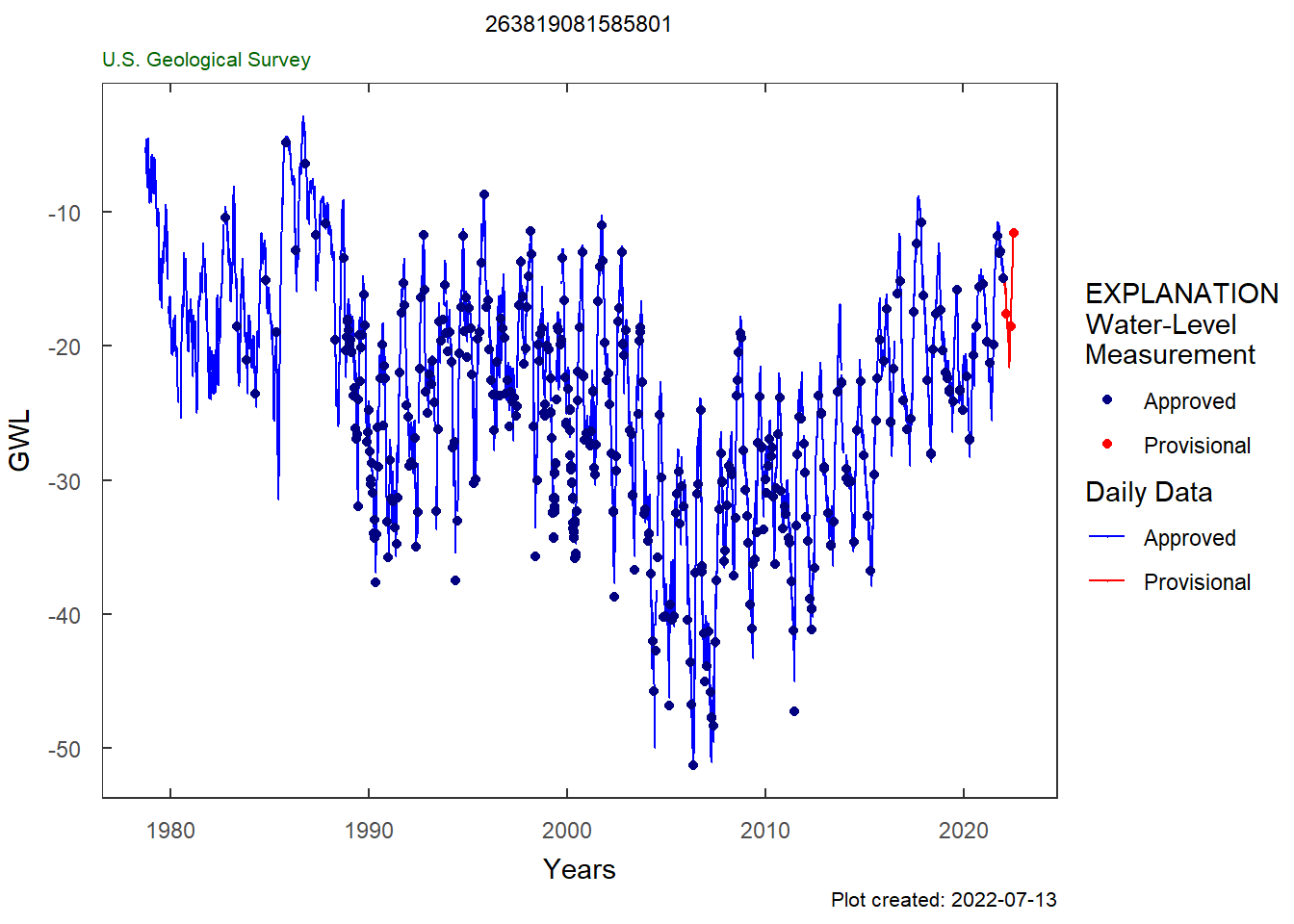
Users can download the aggregated record and see basic statistics that have been calculated with these data. Users also can specify if they should “flip” the y-axis when working with groundwater data or other data that should be viewed differently than a traditional y-axis. This is powerful in allowing users to control how these groundwater data are contextualized, especially in understanding what values mean in the subsurface.
| site_no | 263819081585801 |
| min_site | 17.83 |
| max_site | 64.3 |
| mean_site | 39.29886 |
| p10 | 29.575 |
| p25 | 33.2175 |
| p50 | 38.675 |
| p75 | 44.9775 |
| p90 | 49.46 |
| count | 1398 |
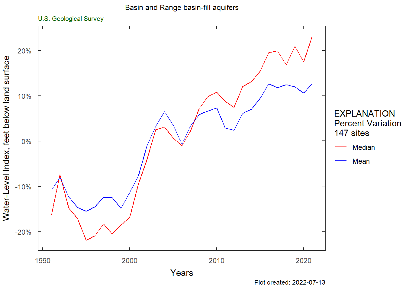
HASP also allows users to plot groundwater level trends in major aquifers as well. The explore_aquifers function allows users to pull data from wells classified in Principal Aquifers and synthesize water-level data to better understand trends. Users can specify a Principal Aquifer and view a map of sites in that aquifer. Users can also view a composite and normalized composite hydrograph for that aquifer for a specified time frame, allowing them to simply view data from many sites in one plot.
library(HASP)
end_date <- "2022-07-08"
state_date <- "1990-12-31"
aquifer_long_name <- "Basin and Range basin-fill aquifers"

aquiferCd <- summary_aquifers$nat_aqfr_cd[summary_aquifers$long_name == aquifer_long_name]

aquifer_data <- get_aquifer_data(aquiferCd,
                                 state_date,
                                 end_date)

plot_normalized_data(aquifer_data,
                     num_years = 30,
                     plot_title = aquifer_long_name)
Enhanced Graphs for Understand Long-Term Trends
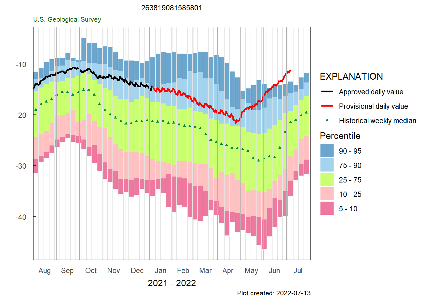
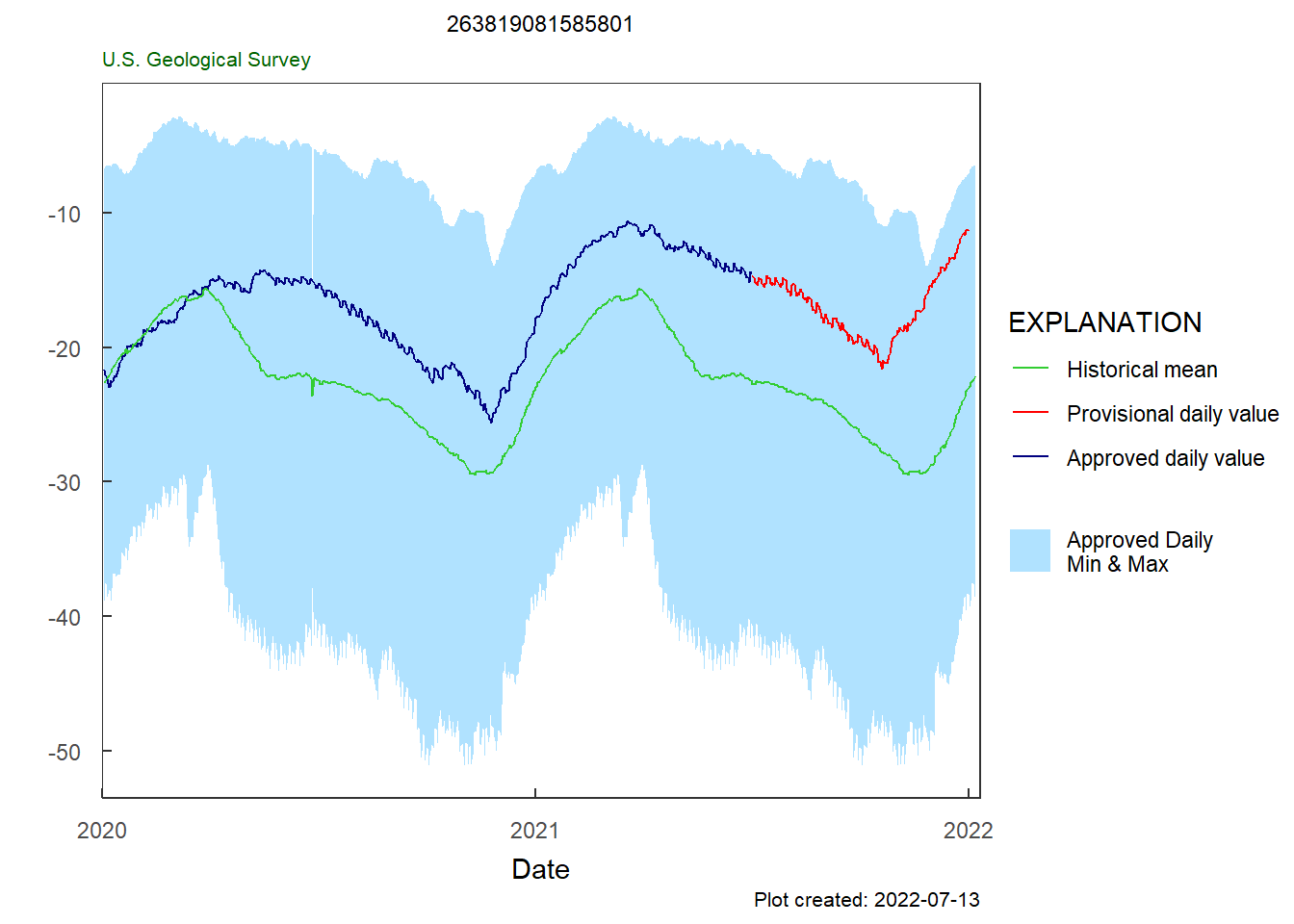
HASP allows users to view aggregated record a weekly view with associated statistics, or in a daily view with associated statistics. These two graphical views put recent groundwater measurements into context by comparing with historical measurements.
weekly_frequency_plot(gw_level_dv = dv,
                      plot_title = site,
                      parameter_cd = pCode)
daily_gwl_2yr_plot(gw_level_dv = dv,
                      plot_title = site,
                      parameter_cd = pCode)
Many users want to understand how recent measurements related to monthly data from past years. HASP also generates a monthly plot along with associated statistics. Many groundwater data users may be familiar with this same graphic that has traditionally been generated by Groundwater Watch.
monthly_frequency_plot(dv,
                       parameter_cd = pCode,
                       plot_title = site,
                       plot_range = "Past year")
monthly_freq_table <- monthly_frequency_table(dv,
                                              parameter_cd = pCode)
kable(monthly_freq_table, digits = 1)
| month | p5 | p10 | p25 | p50 | p75 | p90 | p95 | nYears | minMed | maxMed |
|---|---|---|---|---|---|---|---|---|---|---|
| 1 | -37.9 | -32.4 | -29.0 | -21.4 | -17.7 | -13.8 | -7.9 | 43 | -41.8 | -5.7 |
| 2 | -39.8 | -32.6 | -29.2 | -22.1 | -18.8 | -12.5 | -7.9 | 43 | -42.8 | -7.2 |
| 3 | -40.1 | -36.0 | -29.9 | -24.0 | -20.1 | -12.3 | -8.0 | 43 | -45.1 | -6.9 |
| 4 | -43.2 | -38.9 | -32.2 | -26.2 | -21.9 | -16.3 | -11.2 | 43 | -48.5 | -9.3 |
| 5 | -45.8 | -40.1 | -34.9 | -27.9 | -23.4 | -18.6 | -14.2 | 43 | -49.4 | -10.0 |
| 6 | -41.7 | -37.0 | -32.9 | -26.7 | -21.1 | -16.7 | -14.3 | 42 | -42.8 | -11.0 |
| 7 | -33.1 | -31.1 | -26.3 | -20.5 | -17.7 | -14.5 | -12.1 | 43 | -37.6 | -6.8 |
| 8 | -28.9 | -27.4 | -22.5 | -17.6 | -14.1 | -12.2 | -9.2 | 43 | -32.5 | -4.8 |
| 9 | -25.3 | -24.1 | -19.8 | -15.6 | -12.7 | -9.7 | -8.8 | 42 | -32.5 | -3.2 |
| 10 | -29.2 | -26.5 | -21.3 | -16.2 | -12.6 | -9.6 | -6.1 | 44 | -35.9 | -4.8 |
| 11 | -34.6 | -31.8 | -25.7 | -20.7 | -16.1 | -10.4 | -7.6 | 44 | -41.3 | -4.5 |
| 12 | -35.9 | -32.6 | -27.7 | -21.4 | -16.9 | -13.2 | -9.3 | 43 | -42.4 | -4.9 |
See Changes in Water Quality Over Time
Users can also plot basic water-quality data in HASP. Users can plot chloride concentrations against time and view 5-year trends and 20-year trends in chloride. HASP allows users to generate this plot for any water-quality parameter, so users can quickly and easily view trends of specific analytes over time.
cl_sc <- c("Chloride", "Specific conductance")
qw_data <- qw_data <- readWQPqw(paste0("USGS-", site),
                                cl_sc)
trend_plot(qw_data, plot_title = site)
HASP also generates chloride versus specific conductance plots, which can be useful when examining trends, especially those in coastal areas where saltwater intrusion is a risk.
qw_plot(qw_data, "Specific Conductance",
        CharacteristicName = "Specific conductance")
Moving Beyond Groundwater
HASP uses the dataRetrieval package to retrieve data from USGS sites. Although HASP was written with groundwater data in mind, it can also be used to analyze USGS surface water sites. Users can call data from surface water sites using HASP and access a complete record of all observations at a site over time, helping users to easily access data and statistics over the entire period of observation. If you have thoughts about how we can further enhance this package, email WDFN@usgs.gov .
Disclaimer
Any use of trade, firm, or product names is for descriptive purposes only and does not imply endorsement by the U.S. Government.
Categories:
Related Posts
Large sample pulls using dataRetrieval
July 26, 2022
dataRetrievalis an R package that provides user-friendly access to water data from either the Water Quality Portal (WQP) or the National Water Information Service (NWIS).dataRetrievalmakes it easier for a user to download data from the WQP or NWIS and convert it into usable formats.Tutorial of dataRetrieval's newest features in R
November 26, 2025
This article will describe the R-package
dataRetrieval, which simplifies the process of finding and retrieving water from the U.S. Geological Survey (USGS) and other agencies. We have recently released a new version ofdataRetrievalto work with the modernized Water Data APIs . The new version ofdataRetrievalhas several benefits for new and existing users:Reproducible Data Science in R: Say the quiet part out loud with assertion tests
September 2, 2025

Overview
This blog post is part of the Reprodicuble data science in R series that works up from functional programming foundations through the use of the targets R package to create efficient, reproducible data workflows.
Duplicating Quarto elements with code templates to reduce copy and paste errors
May 20, 2025
Introduction
It is a common situation in data science and analysis: We want to create a series of figures, tables, or summary statistics for a set of data. Maybe we’re studying different species of irises or penguins or the current flow conditions for various streamgages (the example used below), and we want a different summary figure or table for each. One common approach is to write code for one set of the data, such as setting up the graphing parameters in a
ggplotdata visualization or calculating a series of statistics for a single species/streamgage. Then, once happy with that, copying and pasting the code for each entity, modifying the code slightly for each iteration.Formatting guidance for USGS Samples Data Tables
May 6, 2025
Recently, changes were made to the delivery format of USGS samples data (learn more here ). In this blog, we describe the impact to users and show an example of how to use R to convert WQX-formatted water quality results data to a tabular, or “wide” view.