
Maps with inlmisc
Using the R-package inlmisc to create static and dynamic maps.
Introduction
This document gives a brief introduction to making static and dynamic maps using inlmisc, an R package developed by researchers at the United States Geological Survey (USGS) Idaho National Laboratory (INL) Project Office. Included with inlmisc is a collection of functions for creating high-level graphics, such as graphs, maps, and cross sections. All graphics attempt to adhere to the formatting standards for illustrations in USGS publications. You can install the package from CRAN using the command:
if (system.file(package = "inlmisc", lib.loc = .libPaths()) == "")
  utils::install.packages("inlmisc", dependencies = TRUE)
Static Maps
Let’s begin by transforming the now famous meuse data set, introduced by Burrough and McDonnell (1998), into a static map. First define a georeferenced raster layer object from the point data of top soil zinc concentrations.
data(meuse, meuse.grid, package = "sp")
sp::coordinates(meuse.grid) <- ~x+y
sp::proj4string(meuse.grid) <- sp::CRS("+init=epsg:28992")
sp::gridded(meuse.grid) <- TRUE
meuse.grid <- raster::raster(meuse.grid, layer = "soil")
model <- gstat::gstat(id = "zinc", formula = zinc~1, locations = ~x+y, data = meuse)
r <- raster::interpolate(meuse.grid, model)
r <- raster::mask(r, meuse.grid)
Next, plot a map from the gridded data and include a scale bar and vertical legend.
Pal <- function(n) inlmisc::GetTolColors(n, start=0.3, end=0.9)  # color palette
breaks <- seq(0, 2000, by = 200)  # break points used to partition colors
credit <- paste("Data collected in a flood plain of the river Meuse,",
                "near the village of Stein (Netherlands),",
                "\nand iterpolated on a grid with 40-meter by 40-meter spacing",
                "using inverse distance weighting.")
inlmisc::PlotMap(r, breaks = breaks, pal = Pal, dms.tick = TRUE, bg.lines = TRUE,
                 contour.lines = list(col = "#1F1F1F"), credit = credit,
                 draw.key = FALSE, simplify = 0)
inlmisc::AddScaleBar(unit = c("KILOMETER", "MILES"), conv.fact = c(0.001, 0.0006214),
                     loc = "bottomright", inset = c(0.12, 0.05))
inlmisc::AddGradientLegend(breaks, Pal, at = breaks,
                           title = "Topsoil zinc\nconcentration\n(ppm)",
                           loc = "topleft", inset = c(0.05, 0.1),
                           strip.dim = c(2, 20))
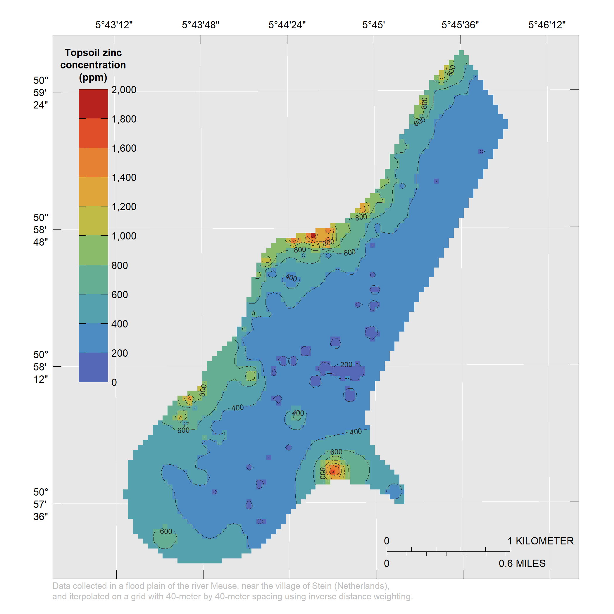
Static map of meuse data set.
For the next example, transform Auckland’s Maunga Whau volcano data set into a static map. First define a georeferenced raster layer object for the volcano’s topographic information.
m <- t(datasets::volcano)[61:1, ]
x <- seq(from = 6478705, length.out = 87, by = 10)
y <- seq(from = 2667405, length.out = 61, by = 10)
r <- raster::raster(m, xmn = min(x), xmx = max(x), ymn = min(y), ymx = max(y),
                    crs = "+init=epsg:27200")
Next, plot a map from the gridded data and include a color key beneath the plot region.
credit <- paste("Digitized from a topographic map by Ross Ihaka",
                "on a grid with 10-meter by 10-meter spacing.")
explanation <- "Elevation on Auckland's Maunga Whau volcano, in meters."
inlmisc::PlotMap(r, xlim = range(x), ylim = range(y), extend.z = TRUE,
                 pal = terrain.colors, explanation = explanation, credit = credit,
                 shade = list(alpha = 0.3), contour.lines = list(col = "#1F1F1F"),
                 useRaster = TRUE)
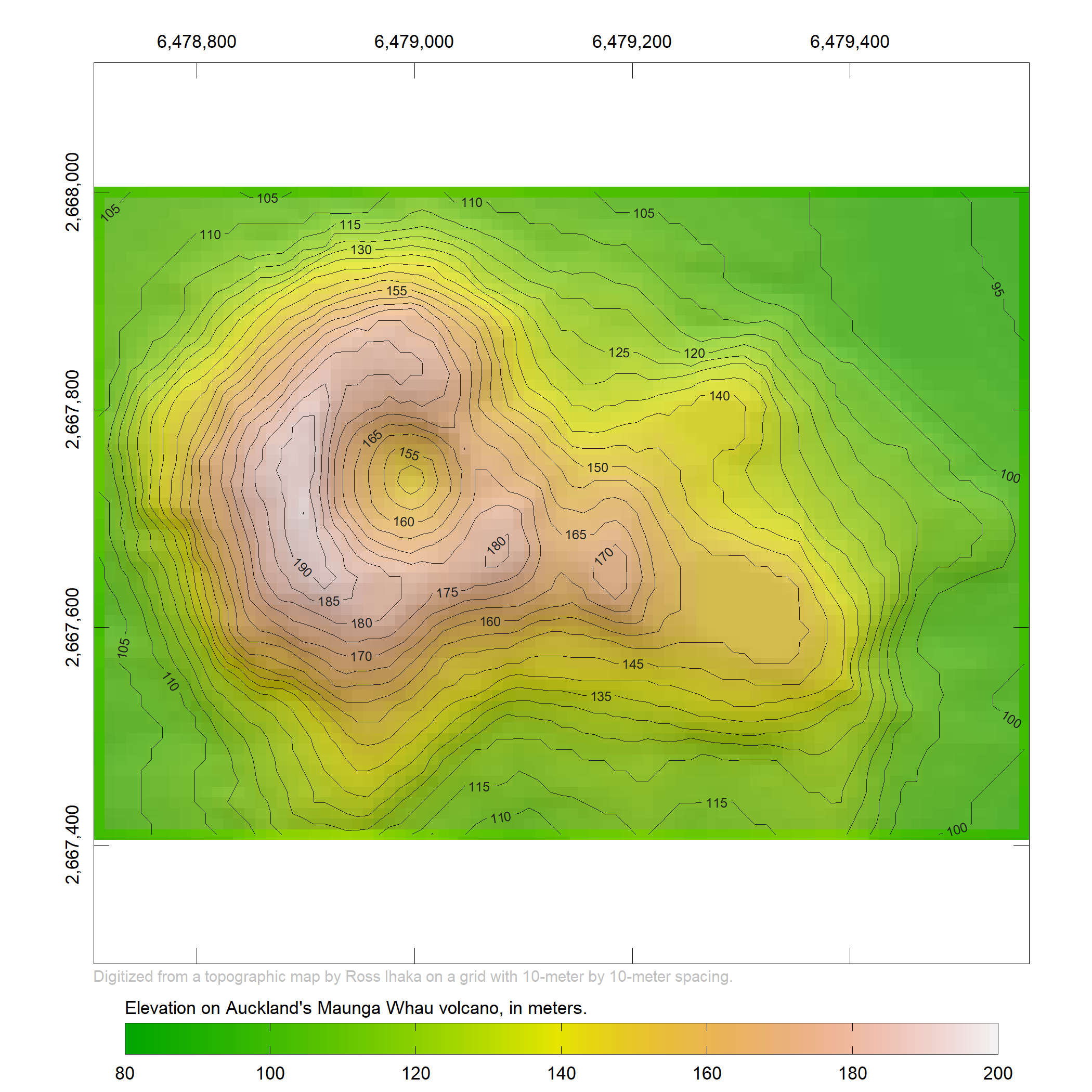
Static map of valcano data set.
One thing you may have noticed is the white space drawn above and below the raster image. White space that results from plotting to a graphics device using the default device dimensions for the canvas of the plotting window (typically 7 inches by 7 inches). Because margin sizes are fixed, the width and height of the plotting region are dependent on the device dimensions—not the data.
If a publication-quality figure is what you’re after,
never use the default values for the device dimensions.
Instead, have the PlotMap function return the dimensions that are optimized for the data.
To do so, specify an output file using the file argument.
The file’s extension determines the format type (only PDF and PNG are supported).
The maximum device dimensions are constrained using the max.dev.dim argument—a
vector of length 2 giving the maximum width and height for the graphics device in picas.
Where 1 pica is equal to 1/6 of an inch, 4.23 millimeters, or 12 points.
Suggested dimensions for single-column, double-column, and sidetitle figures are
c(21, 56), c(43, 56) (default), and c(56, 43), respectively.
out <- inlmisc::PlotMap(r, xlim = range(x), ylim = range(y), extend.z = TRUE,
                        pal = terrain.colors, explanation = explanation,
                        credit = credit, shade = list(alpha = 0.3),
                        contour.lines = list(col = "#1F1F1F"),
                        useRaster = TRUE, file = tempfile(fileext = ".png"))
din <- round(out$din, digits = 2)
cat(sprintf("width = %s, height = %s", din[1], din[2]))
## width = 7.16, height = 5.52
Replotting the map using the returned device dimensions results in a figure that is void of extraneous white space.
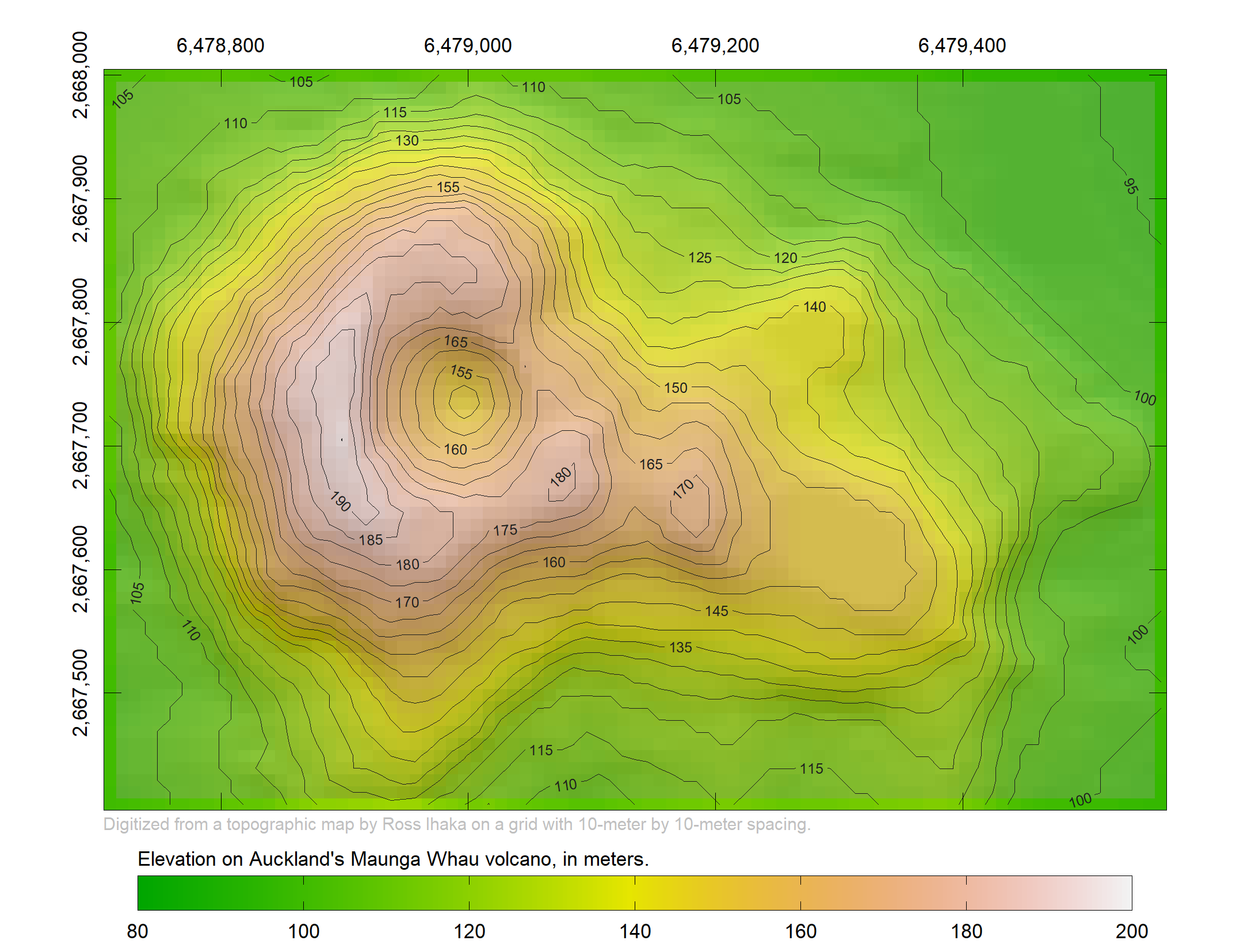
Static map of valcano data set with improved device dimensions.
Dynamic Maps
A dynamic map is an interactive display of geographic information that is powered by the web.
Interactive panning and zooming allows for an explorative view of a map area.
Use the CreateWebMap function to make a dynamic map object.
map <- inlmisc::CreateWebMap()
This function is based on Leaflet for R with base maps provided by The National Map (TNM) services and displayed in a WGS 84 / Pseudo-Mercator (EPSG:3857) coordinate reference system. Data from TNM is free and in the public domain, and available from the USGS, National Geospatial Program.
As an example, transform U.S. city location data into a dynamic map. First define a georeferenced spatial points object for U.S. cities.
city <- rgdal::readOGR(system.file("extdata/city.geojson", package = "inlmisc")[1])
The city data was originally extracted from the Census Bureau’s MAF/TIGER database. Next, add a layer of markers to call out cities on the map, and buttons that may be used to zoom to the initial map extent, and toggle marker clusters on and off. Also add a search element to locate, and move to, a marker.
opt <- leaflet::markerClusterOptions(showCoverageOnHover = FALSE)
map <- leaflet::addMarkers(map, label = ~name, popup = ~name, clusterOptions = opt,
                           clusterId = "cluster", group = "marker", data = city)
map <- inlmisc::AddHomeButton(map)
map <- inlmisc::AddClusterButton(map, clusterId = "cluster")
map <- inlmisc::AddSearchButton(map, group = "marker", zoom = 15,
                                textPlaceholder = "Search city names...")
Print the dynamic map object to display it in your web browser.
print(map)
Some users have reported that base maps do not render correctly in the RStudio viewer. Until RStudio can address this issue, the following workaround is provided.
options(viewer = NULL); print(map)
Let’s take this example a step further and embed the dynamic map within a standalone HTML document. You can share this HTML document just like you would a PDF document. Making it suitable for an appendix in an USGS Scientific Investigation Report.
Before getting started, a few more pieces of software are required. If not already installed, download and install the universal document converter pandoc. The pandoc installer is robust and does not require administrative privileges. R Markdown is also required and used to render a R Markdown document to a HTML document. The R-markdown document is a text file that has the extension ‘.Rmd’ and contains R-code chunks and markdown text. You can install the R-package rmarkdown using the command:
if (system("pandoc -v") == "") warning("pandoc not available")
if (!inlmisc::IsPackageInstalled("rmarkdown"))
  utils::install.packages("rmarkdown")
Let’s also install the R-package leaflet.extras to provide extra functionality for the leaflet R package.
if (!inlmisc::IsPackageInstalled("leaflet.extras"))
  utils::install.packages("leaflet.extras")
Next, create a R Markdown document in your working directory. The document contains a block of R-code with instructions for creating the dynamic map and adding a fullscreen control button.
file <- file.path(getwd(), "example.Rmd")
cat("# Example", "", "```{r out.width = '100%', fig.height = 6}",
    "map <- inlmisc::CreateWebMap(options = leaflet::leafletOptions(minZoom = 2))",
    "map <- leaflet.extras::addFullscreenControl(map, pseudoFullscreen = TRUE)",
    "map", "```", file = file, sep = "\n")
file.show(file)
Note that the R Markdown document is typically created in a text editor. Finally, render the document and view the results in a web browser.
rmarkdown::render(file, "html_document", quiet = TRUE)
utils::browseURL(sprintf("file://%s", file.path(getwd(), "example.html")))
References Cited
Burrough, P.A., and McDonnell, R.A., 1998, Principles of Geographical Information Systems (2d ed.): Oxford, N.Y., Oxford University Press, 35 p.
Reproducibility
R-session information for content in this document is as follows:
##  setting  value
##  version  R version 3.5.1 (2018-07-02)
##  system   x86_64, mingw32
##  ui       Rgui
##  language (EN)
##  collate  English_United States.1252
##  tz       America/Los_Angeles
##  date     2018-09-10
##
##  package        * version date       source
##  backports        1.1.2   2017-12-13 CRAN (R 3.5.0)
##  base           * 3.5.1   2018-07-02 local
##  checkmate        1.8.5   2017-10-24 CRAN (R 3.5.1)
##  compiler         3.5.1   2018-07-02 local
##  crosstalk        1.0.0   2016-12-21 CRAN (R 3.5.1)
##  datasets       * 3.5.1   2018-07-02 local
##  devtools         1.13.6  2018-06-27 CRAN (R 3.5.1)
##  digest           0.6.16  2018-08-22 CRAN (R 3.5.1)
##  evaluate         0.11    2018-07-17 CRAN (R 3.5.1)
##  FNN              1.1.2.1 2018-08-10 CRAN (R 3.5.1)
##  graphics       * 3.5.1   2018-07-02 local
##  grDevices      * 3.5.1   2018-07-02 local
##  grid             3.5.1   2018-07-02 local
##  gstat            1.1-6   2018-04-02 CRAN (R 3.5.1)
##  htmltools        0.3.6   2017-04-28 CRAN (R 3.5.1)
##  htmlwidgets      1.2     2018-04-19 CRAN (R 3.5.1)
##  httpuv           1.4.5   2018-07-19 CRAN (R 3.5.1)
##  igraph           1.2.2   2018-07-27 CRAN (R 3.5.1)
##  inlmisc          0.4.3   2018-09-10 CRAN (R 3.5.1)
##  intervals        0.15.1  2015-08-27 CRAN (R 3.5.0)
##  jsonlite         1.5     2017-06-01 CRAN (R 3.5.1)
##  knitr            1.20    2018-02-20 CRAN (R 3.5.1)
##  later            0.7.4   2018-08-31 CRAN (R 3.5.1)
##  lattice          0.20-35 2017-03-25 CRAN (R 3.5.1)
##  leaflet          2.0.2   2018-08-27 CRAN (R 3.5.1)
##  leaflet.extras   1.0.0   2018-04-21 CRAN (R 3.5.1)
##  magrittr         1.5     2014-11-22 CRAN (R 3.5.1)
##  memoise          1.1.0   2017-04-21 CRAN (R 3.5.1)
##  methods        * 3.5.1   2018-07-02 local
##  mime             0.5     2016-07-07 CRAN (R 3.5.0)
##  pkgconfig        2.0.2   2018-08-16 CRAN (R 3.5.1)
##  promises         1.0.1   2018-04-13 CRAN (R 3.5.1)
##  R6               2.2.2   2017-06-17 CRAN (R 3.5.1)
##  raster           2.6-7   2017-11-13 CRAN (R 3.5.1)
##  Rcpp             0.12.18 2018-07-23 CRAN (R 3.5.1)
##  rgdal            1.3-4   2018-08-03 CRAN (R 3.5.1)
##  rgeos            0.3-28  2018-06-08 CRAN (R 3.5.1)
##  rmarkdown        1.10    2018-06-11 CRAN (R 3.5.1)
##  rprojroot        1.3-2   2018-01-03 CRAN (R 3.5.1)
##  shiny            1.1.0   2018-05-17 CRAN (R 3.5.1)
##  sp               1.3-1   2018-06-05 CRAN (R 3.5.1)
##  spacetime        1.2-2   2018-07-17 CRAN (R 3.5.1)
##  stats          * 3.5.1   2018-07-02 local
##  stringi          1.2.4   2018-07-20 CRAN (R 3.5.1)
##  stringr          1.3.1   2018-05-10 CRAN (R 3.5.1)
##  tools            3.5.1   2018-07-02 local
##  utils          * 3.5.1   2018-07-02 local
##  withr            2.1.2   2018-03-15 CRAN (R 3.5.1)
##  xtable           1.8-3   2018-08-29 CRAN (R 3.5.1)
##  xts              0.11-0  2018-07-16 CRAN (R 3.5.1)
##  yaml             2.2.0   2018-07-25 CRAN (R 3.5.1)
##  zoo              1.8-3   2018-07-16 CRAN (R 3.5.1)
Categories:
Related Posts
The Hydro Network-Linked Data Index
November 2, 2020
Introduction updated 11-2-2020 after updates described here. The Hydro Network-Linked Data Index (NLDI) is a system that can index data to NHDPlus V2 catchments and offers a search service to discover indexed information.
Tol Color Schemes
September 24, 2018
Introduction Choosing colors for a graphic is a bit like taking a trip down the rabbit hole, that is, it can take much longer than expected and be both fun and frustrating at the same time.
The National Map Base Maps
April 12, 2017
A number of map services are offered through The National Map (TNM). There are no use restrictions on these services. However, map content is limited to the United States and Territories.
Furthest Water
September 21, 2018
Finding the Location Furthest from Water in the Conterminous United States The idea for this post came a few months back when I received an email that started, “I am a writer and teacher and am reaching out to you with a question related to a piece I would like to write about the place in the United States that is furthest from a natural body of surface water.
Beyond Basic R - Version Control with Git
August 24, 2018
Depending on how new you are to software development and/or R programming, you may have heard people mention version control, Git, or GitHub. Version control refers to the idea of tracking changes to files through time and various contributors.