Large sample pulls using dataRetrieval

Large pull for all total nitrogen data for streams in the contiguous United States with sites that have at least 40 measurements between 1995 and 2020.

dataRetrieval is an R package that provides user-friendly access to water data from either the Water Quality Portal (WQP) or the National Water Information Service (NWIS). dataRetrieval makes it easier for a user to download data from the WQP or NWIS and convert it into usable formats.

This blog will walk through an example of a large data pull to increase the reusability, reproducibility, and efficiency of WQP data workflows. The script-based workflow uses the WQP summary service to limit the amount downloaded to only relevant data, which can save a lot of time and ultimately reduce the complexity of subsequent data processing. This post is an alternative method to the targets workflow presented in Large Data Pulls from WQP - A Pipeline-Based Approach .

Large data example

This blog sets up a scenario to look at all the total nitrogen data measured in streams within the contiguous United States where sites have at least 40 measurements between 1995 and 2020.

Data download

First, set up a loop to find out which sites have the required data, then get only the data that is relevant.

There are several ways to break up the geographic part of the query, such as bounding box, state, county, or hydrologic unit code (HUC). Depending on the density of the data, it may be ideal to adjust how to loop through the geographic query. Sometimes running a single dataRetrieval call comes back with a “timeout” error. Other times, requests for data spans more than traditional geographic filters of HUC, state, or county. In these cases, it may be necessary to break up the dataRetrieval call into smaller subsets, and then bind those subsets together separately. This blog will discuss one strategy for breaking up a WQP request.

dataRetrieval includes a data frame “stateCd” that has all of the states and territories that could be queried by either NWIS or WQP. In this example, only the lower 48 states along with Washington, D.C.are considered.

Use the readWQPsummary function, which is a very useful function that returns information about all the data that is available for a particular query. The initial query is asking what nitrogen data for streams is available in a particular state. The returned data shows how many nitrogen samples are available at each site for each year. Then, using filtering and summaries will figure out exactly which sites meet the set up scenairo’s needs.

The readWQPdata function is used to download the actual relevant data. This example saves the data using the saveRDS function for each individual state. This ensures higher likelihood of successful completion of the query. For example, if a failure occurs during the download and the loops don’t finish. In that case, the states that successfully downloaded the data are skipped, and only re-run the states that didn’t work. Saving as an “RDS” file also has the benefits of retaining all the attributes of the data. Notice another feature of this loop is using tryCatch for each of the dataRetrieval calls. This allows the loop to continue even if one of the states failed for some reason.

# Load packages
library(dataRetrieval)
library(tidyverse)

state_cd_cont <- stateCd[c(2,4:12,14:52),] # state code information for the 48 conterminous United States plus DC
rownames(state_cd_cont) <- seq(length=nrow(state_cd_cont)) # reset row sequence

for(i in seq_len(nrow(state_cd_cont))){
  
  state_cd <- state_cd_cont$STATE[i]
  state_nm <- state_cd_cont$STUSAB[i]
  message("Getting: ", state_nm)
  
  df_summary <- tryCatch({
    readWQPsummary(statecode = state_cd,
                   CharacteristicName = "Nitrogen",
                   siteType = "Stream")
  }, 
  error=function(cond) {
    message(paste("No data in:", state_nm))
    break()
  })
  
  sites <- df_summary |> 
    filter(YearSummarized >= 1995,
           YearSummarized <= 2020) |> 
    group_by(MonitoringLocationIdentifier, MonitoringLocationName) |> 
    summarise(start_year = min(YearSummarized, na.rm = TRUE),
              end_year = max(YearSummarized, na.rm = TRUE),
              count_activity = sum(ActivityCount, na.rm = TRUE),
              count_result = sum(ResultCount, na.rm = TRUE)) |> 
    ungroup() |> 
    filter(count_activity >= 40)
  
  if(nrow(sites) > 0){
    df_state <- tryCatch({
      readWQPdata(siteid = sites$MonitoringLocationIdentifier,
                  CharacteristicName = "Nitrogen",
                  startDateLo = "1995-01-01",
                  startDateHi = "2020-12-31",
                  sampleMedia = "Water", 
                  ignore_attributes = FALSE)
      # turning off attributes speeds things
      # up, but then you'll need to do the site info later.
      # But...you'll have filtered the number of sites down.
      # If you think that'll be a lot of sites filtered out, 
      # set ignore_attributes to TRUE
    }, 
    error=function(cond) {
      message(paste("No data in:", state_nm))
    })
  }
  
  if(nrow(df_state) > 0){
    
    # I would write the data here, just in case:
    saveRDS(df_state, file = paste0(state_nm, "_raw_data.rds"))
    # You could slim it down here,
    # but if later you decide you wanted something you filtered
    # out here, you'd need to remember to get the data again
    # For example:
    df_state2 <- df_state |> 
      filter(ResultSampleFractionText == "Total") |> 
      group_by(MonitoringLocationIdentifier) |> 
      mutate(count = n()) |> 
      filter(count > 40) |> 
      ungroup()
    
    
  } else {
    message("No data in:", state_nm)
  }
  
  
}

The following can be included in the loop above, but saving it for later allows for more flexibility with the raw data (e.g., leaving data in or filtering data out).

Although creating an empty data frame and filling the data in later would be the most efficient way to go, binding the rows is flexible and easy to conceptualize. For this data download scenario, there wasn’t a huge bottleneck by using the “dyplr::bind_rows”, but that could be a place to reconsider if the next section seems to be taking too long, in which creating the empty data frame may be the considered solution.

The next loop shown below opens each file, pulls out the data we need for analysis, and binds up each state into one large data frame. Notice “ResultMeasureValue” changes into a character vector. By default, dataRetrieval will try to convert that column into numeric. Sometimes however, that can’t be done because there are actual character values in the results. Therefore, to retain all of that information, be sure each state’s “ResultMeasureValue” column is a character (more information on this is below).

all_nitrogen <- data.frame()
# for(state in stateCd$STUSAB){
for(state in state_cd_cont$STUSAB){
  state_df <- tryCatch({
    readRDS(paste0(state, "_raw_data.rds"))
  })
  if(nrow(state_df) > 0){
    df_slim <- state_df |>
      mutate(ResultMeasureValue = as.character(ResultMeasureValue),
             `DetectionQuantitationLimitMeasure.MeasureValue` = as.character(`DetectionQuantitationLimitMeasure.MeasureValue`)) |>
      filter(ActivityMediaSubdivisionName %in%
               c("Surface Water")|
               is.na(ActivityMediaSubdivisionName),
             ResultSampleFractionText %in% c("Total")) |>
      left_join(attr(state_df, "siteInfo") |>
                  select(MonitoringLocationIdentifier,
                         dec_lat_va, dec_lon_va,
                         MonitoringLocationName,
                         MonitoringLocationTypeName,
                         HUCEightDigitCode),
                by = "MonitoringLocationIdentifier")
    
    all_nitrogen <- bind_rows(all_nitrogen, df_slim)
  }
  
}

Results can be provided in a non-numeric format (e.g. “no data”, “bdl”, “<0.1”), which is why it is important to keep the result in character form:

unique(all_nitrogen$ResultMeasureValue[which(!is.na(all_nitrogen$ResultMeasureValue) &
                                        is.na(as.numeric(all_nitrogen$ResultMeasureValue)))])

##  [1] "N/A"                    "no data"                "bdl"                   
##  [4] "BDL"                    "below detection limits" "..198"                 
##  [7] "*Non-detect"            "0,8"                    "<0.50000000"           
## [10] ">0.00000000"            "<1.00000000"            "<0.05000000"           
## [13] "<0.00000000"

Explore the output

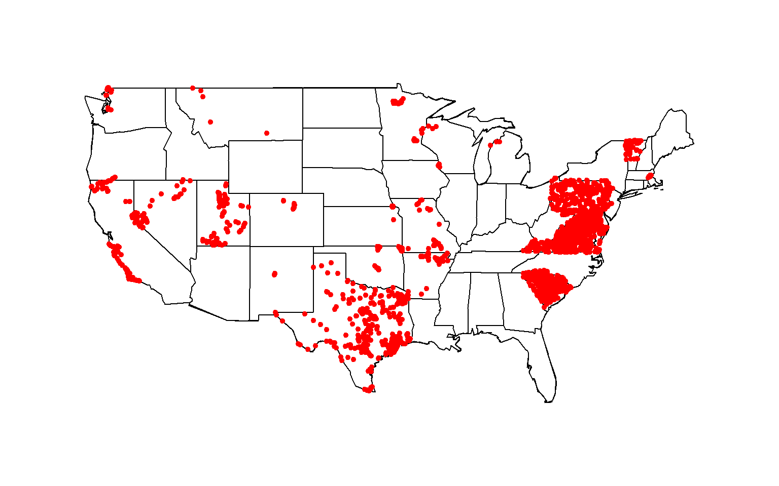
Visually view the data available

To identify the geospatial footprint of sites that meet the above data download criteria, create a map showing all site locations. Here, the maps package is used to create the base map of the conterminous United States, fills in state outlines, and draws the site locations using the latitude and longitude coordinates from the data download.

# Load packages
library(maps)

# create the base map so that map extents are correct
map("usa")

# add state outlines
map("state", add=TRUE)

# draw the site locations onto th map
points(all_nitrogen$dec_lon_va, all_nitrogen$dec_lat_va, col="red", pch=20)

Data exploration and data filtering

Depending on the purpose of the data, non-numeric result values may or may not be useful. Although total nitrogen standards differ between states, suppose your purpose is to compare total nitrogen data among sites between 1995 and 2020 to the U.S. Environmental Protection Agency (EPA) total nitrogen acceptable range of 2-6 milligrams per liter (mg/l; U.S. Environmental Protection Agency, 2013). With this defined purpose, you would be looking at field data with known concentrations. In order to compare the data to the EPA acceptable range, the data would need to be in mg/l.

Reference: U.S. Environmental Protection Agency, 2013, Total Nitrogen - Revised: EPA 090-R-090-20A.

First, explore the unique sample types:

# determine sample types
unique(all_nitrogen$ActivityTypeCode)

##  [1] "Sample-Routine"                                      
##  [2] "Quality Control Sample-Field Blank"                  
##  [3] "Sample-Field Split"                                  
##  [4] "Field Msr/Obs"                                       
##  [5] "Sample-Other"                                        
##  [6] "Quality Control Sample-Field Replicate"              
##  [7] "Quality Control Sample-Blind Duplicate"              
##  [8] "Quality Control Sample-Equipment Blank"              
##  [9] "Sample-Field Subsample"                              
## [10] "Quality Control Sample-Lab Duplicate"                
## [11] "Sample-Integrated Vertical Profile"                  
## [12] "Quality Control Sample-Inter-lab Split"              
## [13] "Quality Control Field Sample Equipment Rinsate Blank"
## [14] "Sample-Composite Without Parents"                    
## [15] "Field Msr/Obs-Habitat Assessment"                    
## [16] "Sample-Integrated Cross-Sectional Profile"           
## [17] "Sample-Integrated Horizontal Profile"                
## [18] "Sample-Integrated Time Series"

Second, explore the reported result units:

# determine units used to report total nitrogen
unique(all_nitrogen$ResultMeasure.MeasureUnitCode)

## [1] "mg/l"      "ppm"       NA          "ug/l"      "MPN/100ml" "ug"

In the above two snippet of code and output, you see there are field and quality assurance data reported in a variety of units.

Third, use piping (%>%) and the filter function from the dplyr package to filter out quality assurance data and then filter result units in weight per unit volume of water.

# filter out quality control data by using the "filter" function, and then use the "filter" function again to keep only results reported in wight per unit volume of water.
all_nitrogen <- all_nitrogen %>% 
  filter(!grepl("Quality Control", ActivityTypeCode)) %>% 
  filter(ResultMeasure.MeasureUnitCode=="mg/l" |  ResultMeasure.MeasureUnitCode=="ppm" |                              ResultMeasure.MeasureUnitCode=="ug/l")  

In the above snippet of code, the pipe operator (%>%) takes the output of the first function in front of it and passes it to the second function, which allows you to express a sequence of multiple operations.

Now, explore the non-numeric result values. Here, create a new data frame “nonnum” using piping and the filter function again to filter non-numeric result values that are also not reported as NA.

nonnum <- all_nitrogen %>% 
  filter(ResultMeasureValue %>% 
           as.numeric() %>% 
           is.na())

Viewing the “nonnum” data frame, some result values were reported as censored with a “<” or “>” character or simply appear to have been entered with typos (i.e., “..198 and 0,8), while other result values are reported as censored below the detection limit (i.e.,”bdl”, “BDL”, “below detection limits”) or no data reported (i.e., “N/A”, “no data”, or NA). With that, the user would have to make decisions on how to use these data.

Next, explore the non-numeric result values. Create a new data frame named “nitrogen” with only pertinent columns to make the data easier to work with. Then, create a new column of result values named “Result”. The purpose of creating a new results column is to retain the original results data while still being able work with the data (unit conversions, non-numeric to numeric, etc.).

# create a new data frame with only pertinent columns from the existing all_nitrogen data frame
nitrogen <- all_nitrogen[,c("OrganizationIdentifier", "OrganizationFormalName", "ActivityIdentifier", "ActivityTypeCode", "ActivityStartDate", "ActivityCommentText", "ResultDetectionConditionText", "CharacteristicName", "ResultSampleFractionText", "ResultMeasureValue", "ResultMeasure.MeasureUnitCode", "MeasureQualifierCode", "ResultStatusIdentifier", "ResultValueTypeName", "ResultCommentText", "ResultLaboratoryCommentText", "DetectionQuantitationLimitTypeName", "DetectionQuantitationLimitMeasure.MeasureValue", "DetectionQuantitationLimitMeasure.MeasureUnitCode", "dec_lat_va", "dec_lon_va", "MonitoringLocationName", "MonitoringLocationIdentifier", "MonitoringLocationTypeName")]

# create new Result column using the original result value column
nitrogen$Result <- nitrogen$ResultMeasureValue

Then, for result values reported as censored or below the detection limit, create a new column named “ResultComment” to retain the censored information.

# create a new column to retain result value censoring information
nitrogen <-
  nitrogen %>% mutate(ResultComment=
                        case_when(grepl("<", Result) ~ "<",
                                  grepl(">", Result) ~ ">",
                                  grepl("BDL", Result) ~ "<",
                                  grepl("bdl", Result) ~ "<",
                                  grepl("below detection limits", Result) ~ "<",
                                  grepl("Not Detected", ResultDetectionConditionText) ~ "<",
                                  grepl("Present Below Quantification Limit",  ResultDetectionConditionText) ~ "<"))

Censored data are still useful for the purpose of this analysis. If a value was originally reported below a certain known threshold below the threshold of this analysis (2 mg/l), the result can still be used at that value. Now, some values that are censored do not provide the censoring limit in the results value column, but some results provide a censor threshold in the “DectectionQuantitationLimitMeasure.MeasureValue” column. In these instances, pull this information into the results column. Then, remove “<” or “>” from the “Result” column since the censoring of these data have been retained in the “ResultComment” column created in the last snippet of code.

Again, using piping, if available, fill NA result values with a censored result comment with the censoring threshold while retaining the result values that are not censored. Then, remove the “<” or “>” characters from the result column.

nitrogen <-
  nitrogen %>% mutate(Result=
  case_when(is.na(Result) & ResultComment=="<" ~ DetectionQuantitationLimitMeasure.MeasureValue, 
            !is.na(Result) ~ Result))


# remove censoring from Result column
nitrogen$Result <- gsub("<", "",
                   gsub(">", "", nitrogen$Result)) 

In the above first snippet of code, if the “Result” column is NA and the “ResultComment” column contains a “<” then, if reported, the detection limit is made the “Result” column value. While, if the “Result” column value is already provided, the result value remains the same.

Next, filter out the remaining non-numeric values that do not provide a numeric result value, including values that seem to be typos. These values should be removed because they cannot be used to compare results to the EPA acceptable range for total nitrogen (2-6 mg/l). Lastly, change the data format to numeric form. Data are converted to numeric form for unit conversions.

# filter out non-numeric values
nitrogen <-
  nitrogen %>% 
    filter(!grepl("no data|N/A|0,8|..198|-", Result)) %>%
    mutate(Result = as.numeric(Result)) 

There are still NA result values reported that do not indicate it is censored or is censored and does not provide a censoring threshold, so these values are not useful for this analysis and should be filtered out.

# remove NA result values
nitrogen <- nitrogen %>%
  filter(!is.na(Result))    

Lastly, convert all results to mg/l. Some results are already in mg/l and 1 part per million (ppm) is approximately equivalent to 1 mg/l, so these results do not need to be converted. Result values reported in micrograms per liter (ug/l) should be divided by 1000 to convert to mg/l.

# convert values to single units (milligrams per liter)
nitrogen <-
  nitrogen %>% mutate(Result_mgL=
                case_when(ResultMeasure.MeasureUnitCode=="ug/l" ~ Result/1000, 
                          ResultMeasure.MeasureUnitCode=="mg/l" ~ Result, 
                          ResultMeasure.MeasureUnitCode=="ppm" ~ Result)) 

Summarize data

The data shows there are multiple results per site per year. Let’s say the goal is to calculate the annual mean and median total nitrogen values for each site. First, create a new column that extracts just the year from the sample date. Then, group the data by site identifier and location (latitude and longitude) and calculate the mean and median for each year.

# pull the year from the date
nitrogen$year <- format(as.Date(nitrogen$ActivityStartDate, format="%Y-%m-%d"),"%Y")

# create new data frame of summarized result data
n_bysite <- 
  nitrogen %>% 
      group_by(MonitoringLocationIdentifier, dec_lat_va, dec_lon_va, year) %>% 
      summarize(mean = mean(Result_mgL), 
                median = median(Result_mgL)) 

Finally, use the total nitrogen annual mean data to create a column called “TN_mean” to indicate if the annual mean is below the EPA acceptable range (<2 mg/l), within the acceptable (2-6 mg/l), or above the acceptable (>6 mg/l).

# create a new character column with total nitrogen acceptable range designations
n_bysite <- 
  n_bysite %>% mutate(TN_mean=
                        case_when(mean<2 ~ "<2 mg/l", 
                                  mean>=2 & mean<=6 ~ "2-6 mg/l", 
                                  mean>6 ~ ">6 mg/l")) 

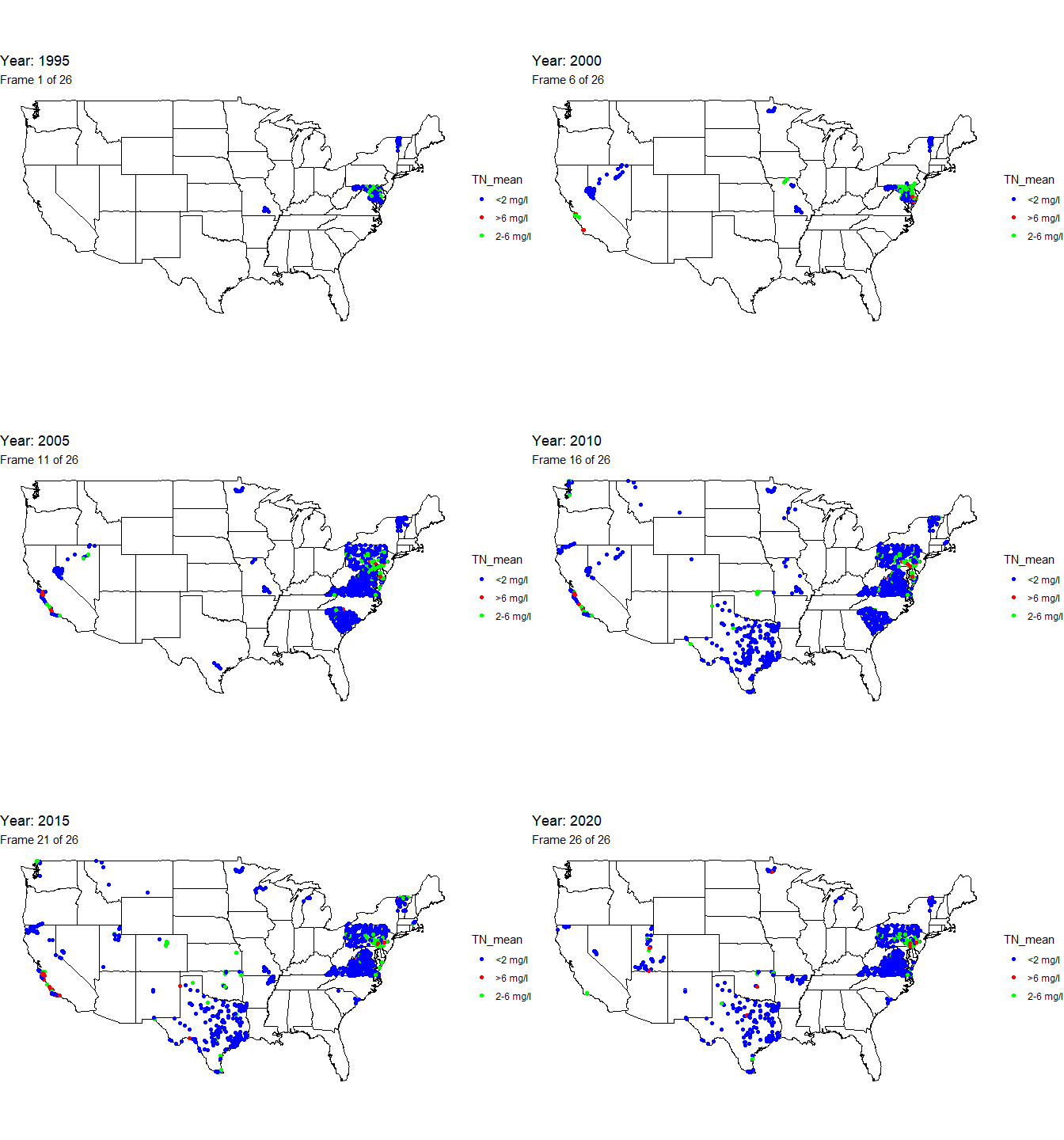
Create animated map

An animation is a powerful visualization tool used to show how data changes over time. Animate the data by year and result value based on EPA acceptable standard range for total nitrogen in streams (2-6 milligrams per liter). Create this animated map using the maps, ggplot2, gganimate, and gifski packages.

First, before plotting out data on to a map, create a data frame that contains the base map. The maps package provides the base map boundary and state outlines, while the map_data function from the ggplot2 package creates the data frame containing the base map data in a data frame. The all_state variable was assigned the map boundary to all states in the contiguous United States. In the base map data frame, the “group” column groups the data by state (e.g., 1 = Alabama, 2 = Arizona).

Second, plot the base map and add the data to it. Here, the base map data that is created is used to plot the base map and the summarized (annual mean) total nitrogen data for each site location. The total nitrogen acceptable range data are assigned to the color parameter and the data are grouped by year for each frame. The transition_time is specified to use the year to move from one frame of the animation to the next.

Lastly, run the animation using the animate function from the gganimate package. Here the number of frame changes are equal the the number of years in the data set.

# Load packages
library(ggplot2)
library(gganimate)
library(gifski)

# convert latitude, longitude, and year data to numeric form
n_bysite$dec_lat_va <- as.numeric(n_bysite$dec_lat_va)
n_bysite$dec_lon_va <- as.numeric(n_bysite$dec_lon_va)
n_bysite$year <- as.numeric(n_bysite$year)

# first, create the base map data frame
all_state <- "usa"
usa <- map_data("state", interior=TRUE)
base_map <- ggplot(data = usa, mapping = aes(x = long, 
                                             y = lat, 
                                             group = group)) +
  geom_polygon(color = "black", fill = "white") +
  coord_quickmap() +
  theme_void() 

# second, plot the base map and add data to it
map_with_data <- base_map +
  geom_point(data = n_bysite, aes(x = dec_lon_va, 
                                  y = dec_lat_va, 
                                  color = TN_mean, 
                                  group = year, 
                                  frame = year)) +
  transition_time(year) +
  ggtitle('Year: {frame_time}', # add year to the title
        subtitle = 'Frame {frame} of {nframes}') +
  scale_colour_manual(values = c("blue", "red", "green")) 
num_years <- max(n_bysite$year)-min(n_bysite$year) + 1 

# lastly, run the animation
animate(map_with_data, nframes = num_years, fps = 1)

The below line of code will save the output gif:

#anim_save("TN.gif", map_with_data, nframes = num_years, fps = 1)  # save

Disclaimer

Any use of trade, firm, or product names is for descriptive purposes only and does not imply endorsement by the U.S. Government.