
Toward a searchable, network-linked database of river inundation extents
This post provides a brief description of work done through fiscal year 2022 for the River Corridors project as part of the National Hydrologic Geospatial Fabric (NHGF) project to create a new database.
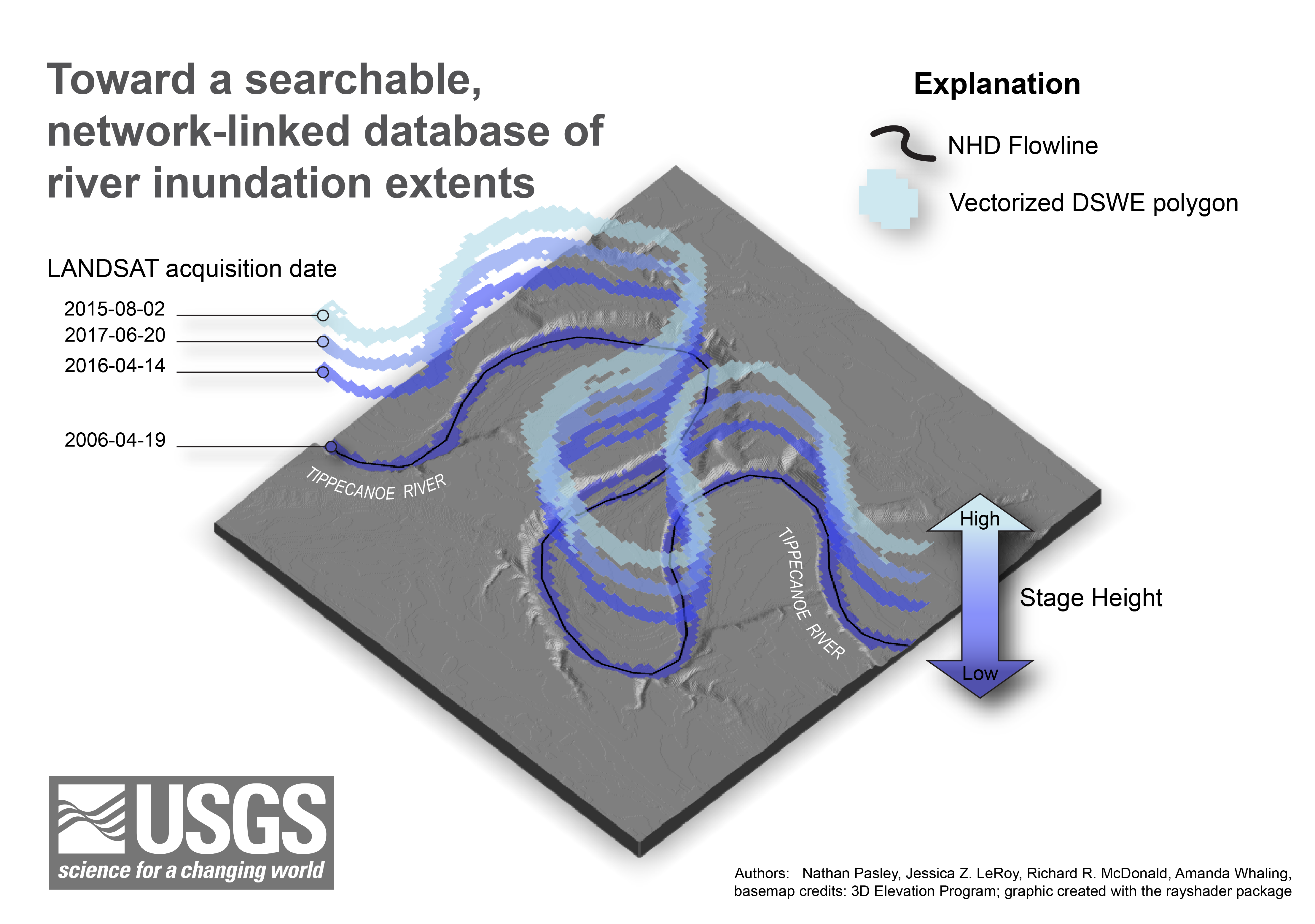
Processed inundation extent polygons for various dates and stage heights of the Tippecanoe River.
Flood inundation mapping (FIM) is typically a hydraulic modeling exercise, requiring detailed topobathymetry, roughness and/or land cover data, boundary conditions, and calibration/validation data. As a result, FIM studies are time and labor intensive and often limited in geographic extent. Remotely sensed imagery of Earth’s surface offers an alternate approach to inundation mapping.
We developed a python workflow to derive river inundation extents using the U.S. Geological Survey (USGS) Landsat Dynamic Surface Water Extent (DSWE)1 collection 2 science product. The Landsat DSWE product provides a unique historical dataset that includes classifications for the presence and absence of surface water throughout the United States. This means the hard part is already done! Our python workflow indexes DSWE-derived inundation extents to National Hydrography Dataset Plus version 2.1 (NHDPlusV2.1)2 using a unique identifier for the stream segment (the COMID) and tags those extents with the imagery acquisition date and, where applicable, stage and discharge.
The long-term goal of this work is to develop a searchable database of inundation extents for the entire contiguous United States. Linking the inundation extents to the NHDPlusV2.1 will make it possible to search the database by location along the network, or geographic bounding box, using the Hydro Network Linked Data Index (NLDI)3, as summarized in Figure 1 below.
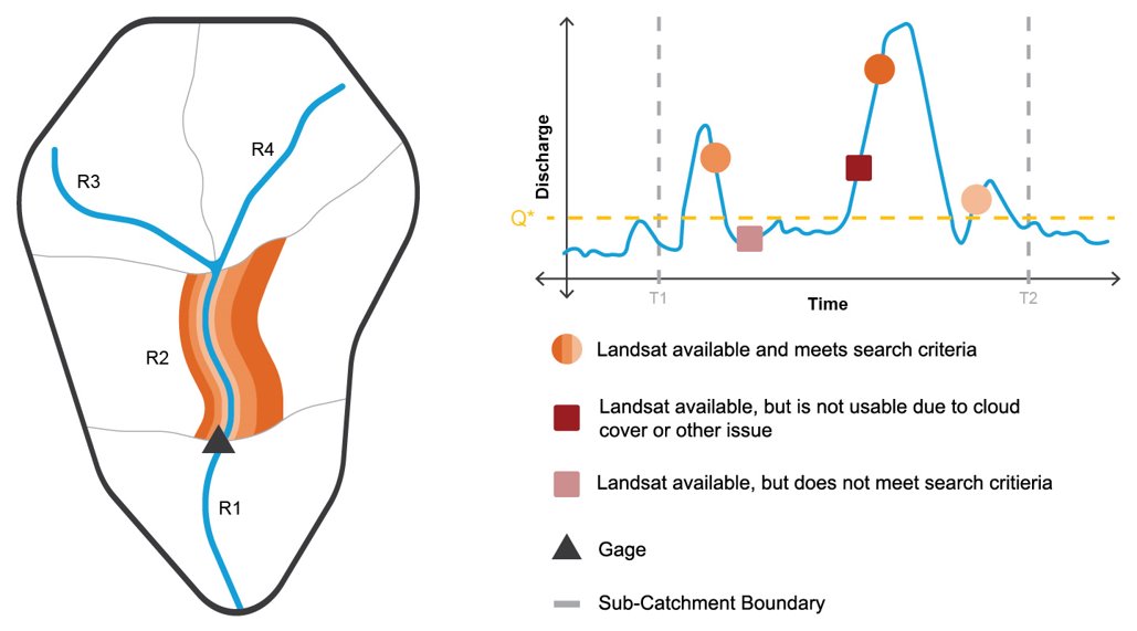
Figure 1. A conceptual diagram illustrating how a database of inundation extents might be used to find the inundation extents for discharges above Q* for segment R2 between times T1 and T2.
This blog post provides an overview of this workflow and its application to a pilot study area along the Wabash River.
Overview of the workflow to create the database
The basic steps of the workflow are to (1) select and download DSWE images, (2) vectorize inundated areas, and (3) index inundation polygons to NHDPlusV2.1. These steps are described in more detail below:
Step 1: Select and download DSWE (Collection 2) images
This step begins with a bulk download of the DSWE metadata for DSWE images within a specified bounding box. Depending on the extent of the area being processed, this bounding box may encompass an area as small as an NHD flowline, a group of NHD catchments, or an entire Landsat tile. Additionally, the stage at the time of image capture is accessed from NWIS for all streamgages within the bounding box. If metadata indicates that the image is relatively cloud-free (in the lower quartile of cloud cover values) and stage values at any of the streamgages indicate high flows (in the upper quartile of stage values), then the image is selected for download. These thresholds are arbitrary but have reduced the number of images to a manageable level (think: tens of thousands of images reduced to tens) while providing sufficient numbers of the best images for times of higher flows. The selected images are then downloaded.
Step 2: Vectorize inundated areas
Individual Landsat pixels within the original DSWE raster have been classified according to the probability of the presence of surface water, as shown in Figure 2b. Our code aggregates and vectorizes all cells excepting those classified as “Not Water” into a single polygon. This step is done using the Python libraries RasterIO, Geopandas, and HyRiver. Much of our effort this year has been applied toward optimizing computation time per DSWE image in this step by using spatial indexing. Currently, this step takes about 50 seconds per image for a full sized DSWE tile. Considering that there are 725 tiles, with each tile containing thousands of DSWE images, having an optimized workflow was of high priority.
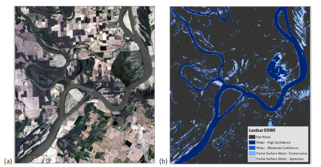
Figure 2. (a) A Landsat Collection 2 U.S. Analysis Ready Data Surface Reflectance image showing the Confluence of the Wabash and Ohio Rivers on April 12, 2021, and (b) A Dynamic Surface Water Extent – Interpreted (INTR) layer showing the DSWE classification of the original Landsat image.
Step 3: Index inundation polygons to NHDPlusV2.1
The inundation polygon is then intersected with the NHDPlusV2.1 catchments, split along those boundaries, and assigned the corresponding COMID attribute, thus linking it to many other useful products like the NHD dataset and NLDI.
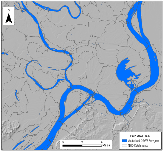
Figure 3. Example of the inundation polygon intersected with NHDPlusV2.1 catchments, where each catchment represents one unique COMID, or stream segment.
Pilot application
We developed the workflow by working with a pilot study area along the Wabash River near Lafayette, IN. We selected this pilot study area because the main channel within it is at least as wide as 30 meters, so as to not cause major issues with respect to the resolution of Landsat, but it also contains smaller tributaries that can be used to test the impacts of that resolution on the output of this workflow. Additionally, there are several streamgages in the area. There is also a traditional USGS FIM study5 for this area that we can compare our result to. We extracted the FIM polygon corresponding to gage height at site number 03335500 on the date and time of each vectorized Landsat capture. On average, derived inundation extents scored a 0.73 and 0.71 in the Lee-Sallee6 and Goodness of Fit7 shape indexes and shared an 84% overlap with the FIM study polygon.
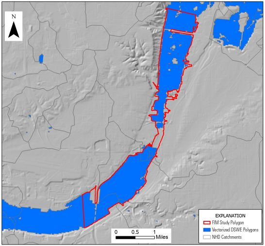
Figure 4. Example comparison of DSWE inundation polygons (in blue) to the FIM study polygon (in red).
Next steps
The primary limitations of using Landsat DSWE for the purposes of this study are its 30-meter resolution and issues of cloud and ice cover. Issues related to cloud cover could be addressed by incorporating synthetic aperture radar (SAR) data into the analysis. SAR sensors emit longer wavelengths at the centimeter to meter scale, thus allowing SAR to capture cloud-free images that may be used to replace areas masked by clouds in certain DSWE images and increase the number of dates depicted in our derived database.
An accompanying dataset featuring channel or centerline may be delineated from the derived polygons in hopes of capturing channel morphology to quantify rates and patterns of lateral migration or changes in channel width or sinuosity. Additionally, a method for extracting water surface elevation using available 3DEP lidar-based digital elevation models (DEM) at vertices of inundation polygons may be explored. Some preliminary testing resulted in water surface elevations within about 0.5 ft of the stage reported at a nearby streamgage and intersecting vertices with a DEM may provide more accurate results. Most importantly, we are looking toward scaling this work up from our pilot study to generate a national scale inundation extent database that could be used for validating model results, examining spatial patterns of wetting and drying and inundation hysteresis during floods, and studying the influence of antecedent conditions on inundation during floods. We would also like to investigate using this pairing of inundation extents and stage to map overbank boundaries and channel centerlines and quantify changes in river planform over time.
With an optimized workflow that’s hungry for data, we are ready to expand the possibilities of current inundation mapping techniques!
Please email npasley@usgs.gov with questions and feedback.
References
1. Landsat collection 2 level-3 dynamic surface water extent science product. (n.d.). Retrieved November 15, 2022, from https://www.usgs.gov/landsat-missions/landsat-collection-2-level-3-dynamic-surface-water-extent-science-product
2. National Hydrography Dataset. (n.d.). Retrieved November 15, 2022, from https://www.usgs.gov/national-hydrography/national-hydrography-dataset
3. Hydro-Network Linked Data index. (2022, October 03). Retrieved November 15, 2022, from https://labs.waterdata.usgs.gov/about-nldi/index.html
4. Example of the landsat collection 2 dynamic surface water extent science product. (n.d.). Retrieved November 15, 2022, from https://www.usgs.gov/media/images/example-landsat-collection-2-dynamic-surface-water-extent-science-product
5. Kim, M.H. (2018) “Flood-inundation maps for the Wabash River at Lafayette, Indiana,” Scientific Investigations Report [Preprint]. Available at: https://doi.org/10.3133/sir20185017.
6. Lee, D. R., & Sallee, G. T. (1970). A method of measuring shape. Geographical Review, 60(4), 555.
https://doi.org/10.2307/213774.
7. Hargrove, W. W., Hoffman, F. M., & Hessburg, P. F. (2006). Mapcurves: A quantitative method for comparing categorical maps. Journal of Geographical Systems, 8(2), 187–208. https://doi.org/10.1007/s10109-006-0025-x.
Categories:
Related Posts
Progress Toward a Reference Hydrologic Geospatial Fabric for the United States
December 12, 2022
This post provides background information for those interested in engaging in use and development of the National Hydrologic Geospatial Fabric (NHGF) Reference and Derived Hydrofabrics provisional data release and the Network Linked Data Index, a search engine built to leverage the NHGF reference hydrofabric.