
Network Linked Data Index (NLDI) Update and Client Applications
An update on the Network Linked Data Index (NLDI) Web Application Programming Interface and Client Applications
In August 2020, the Hydro Network Linked Data Index (NLDI) was updated with new functionality and some changes to the existing Web Application Programming Interface (API). This post summarizes these changes and demonstrates Python and R clients available to work with the functionality.
If you are new to the NLDI, visit the nldi-intro blog to get up to speed. This post assumes a basic understanding of the API.
Summary
The new functionality added to the NLDI retrieves local or accumulated
catchment characteristics for any featureSource. A selection of
characteristics from the this USGS data release are included:
Wieczorek, M.E., Jackson, S.E., and Schwarz, G.E., 2018, Select Attributes for NHDPlus Version 2.1 Reach Catchments and Modified Network Routed Upstream Watersheds for the Conterminous United States (ver. 2.0, November 2019): U.S. Geological Survey data release, https://doi.org/10.5066/F7765D7V .
API changes are backward compatible but significant.
- If using a web-browser,
?f=jsonneeds to be appended to requests to see JSON content. - The
navigateendpoint is deprecated in favor of anavigationend point with modified behavior. – Previously, anavigate/{navigationMode}request would return flowline geometry. Thenavigation/{navigationMode}endpoint now returns availabledataSources, treating flowline geometry as a data source. – AllnavigationModes now require thedistancequery parameter. Unconstrained navigation queries (the default from thenavigateendpoint) were causing system performance problems. Client applications must now explicitly request very large upstream-with-tributaries. - All features in a
featureSourcecan now be accessed at thefeatureSourceendpoint. This will allow clients to easily create map-based selection interfaces. - A
featureSourcecan now be queried with a lat/lon point encoded inWKTformat.
API Updates Detail
The API updates were tracked in a github release here. These updates aimed to make the API more consistent and improve overall scalability of the system. The following sections describe the changes in some detail.
Media type handling changes.
Previous to the recent release, the NLDI only supported JSON responses.
This caused problems in a browser when an unsuspecting person accessed
an API request that returned a large JSON document in a Web browser. To
protect against this, any request from with Accept headers preferring
text/html content (e.g. from a Web browser) is provided an HTML response indicating that an html format is not available and
containing a link to the JSON content. An Accept header override –
?f=json – is used for this behavior. If requests are made without an
Accept header, JSON content is returned.
This behavior can be seen at any endpoint exposed by the NLDI. e.g. open the following url in a browser:
https://api.water.usgs.gov/nldi/linked-data/nwissite/USGS-05429700
Navigation end point.
The original NLDI .../navigate end point had a design inconsistency
and behavior that led to needless high-cost queries. .../navigate has
been deprecated and a .../navigation endpoint has been introduced in
its place.
Flowlines are now a dataSource
The most significant change is the resource returned from a particular navigation mode endpoint.
e.g.
https://api.water.usgs.gov/nldi/linked-data/nwissite/USGS-05429700/navigation/UM
is now a JSON document listing available data sources that can be
accessed for the upstream mainstem (UM) navigation from the featureID
USGS-05429700 from the nwissite featureSource. In contrast, the
.../navigate/UM returns GeoJSON containing flowlines for the upstream
main navigation. The same flowlines GeoJSON is now a dataSource listed
along side the others available for the .../navigation/UM end point.
distance is now a required query parameter
The other significant difference between the .../navigate and
.../navigation endpoints is that the distance (in km) query
parameter is now required. Previously, the internal default was set to
9999 which resulted in many very large requests that may or may not have
been desired. There is no upper limit to the value of the distance
parameter, but it must be provided for the navigation end point to
trigger a query to the NLDI’s database.
Client developers are encouraged to choose a sensible default such that naive users will not accidentally trigger very large queries and be aware that the NLDI is capable of producing result sets with hundreds of thousands of features.
Feature Source Access
Prior to this release, end points such as:
https://api.water.usgs.gov/nldi/linked-data/huc12pp did not
return a resource. This made it difficult to discover available feature
sources. This featureSource end point now returns a GeoJSON document
containing all features from the requested feature source. These are
quite large and no further query functions are implemented. In future
releases, an OGC API Features interface may be made available to allow
queries against the feature sources.
Query by lat/lon
NHDPlusV2 forms the underlying network used by the Network Linked Data Index. NHDPlusV2 catchment polygons are used behind the API to allow a client application to discovery of a catchment id (comid) by providing a lat/lon. The format uses the WKT syntax and is interpreted as NAD83 Lon/Lat.
Requests will look like:
https://api.water.usgs.gov/nldi/linked-data/comid/position?f=json&coords=POINT(-89.35 43.0864)
Catchment Characteristics
The relationship between featureSources that can be accessed in the NLDI and NHDPlusV2 catchments is
important in understanding how the new catchment characteristics functionality works.
All navigation requests resolve to the nearest catchment and an equivalent query can be made directly to the comid that a feature source is indexed to. e.g.
https://api.water.usgs.gov/nldi/linked-data/nwissite/USGS-05429700
is indexed to comid 13297194:
https://api.water.usgs.gov/nldi/linked-data/comid/13297194
so navigation requests starting from either the nwissite or the comid will be equivalent.
Given this, we can access catchment characteristics for a catchment or
an indexed feature with the local, tot, or div end points. e.g.
https://api.water.usgs.gov/nldi/linked-data/comid/13297194/local
or
https://api.water.usgs.gov/nldi/linked-data/nwissite/USGS-05429700/local
provide exactly the same content.
- The
localend point provides characteristics for the local catchment. - The
totend point provides total-upstream characteristics. - The
divend point provides divergence-routed upstream characteristics.
Documentation for the source dataset and creation methods can be found here.
Wieczorek, M.E., Jackson, S.E., and Schwarz, G.E., 2018, Select Attributes for NHDPlus Version 2.1 Reach Catchments and Modified Network Routed Upstream Watersheds for the Conterminous United States (ver. 2.0, November 2019): U.S. Geological Survey data release, https://doi.org/10.5066/F7765D7V .
An endpoint to lookup metadata for specific characteristics is available here:
https://api.water.usgs.gov/nldi/lookups
Only selected catchment characteristics from the source data release are included at this time. More may be added in the future. Please reach out in a github issue here to request additional characteristics be added.
Client Applications
The examples below show two example client applications that work with the NLDI.
PyNHD and nhdplusTools
NOTE: This post was rendered from “R Markdown” into what you are reading using a Docker-based R / Python environment (hydrogeoenv ) that contains dependencies for both these client applications.
Python Client Application
Contributed by Taher Chegini . Thanks!!
Let’s use PyNHD
to demonstrate new
NLDI’s capabilities. Based on a topologically sorted river network
pynhd.vector_accumulation function computes the accumulation of an
attribute in the network. We use the upstream river network of
USGS-01031500 station as an example. This station is located in a
natural watershed and is located in Piscataquis County, Maine with a
drainage area of 298 square miles. First, lets use NLDI’s navigation
end-point to get all its upstream NHDPlus Common Identifiers (ComIDs).
    from pynhd import NLDI, WaterData
    import pynhd as nhd

    nldi = NLDI()
    comids = nldi.navigate_byid(
        fsource="nwissite",
        fid="USGS-01031500",
        navigation="upstreamTributaries",
        source="flowlines",
        distance=1000,
    ).nhdplus_comid.to_list()
Then, we use WaterData GeoServer, which has the same version of the NHD as the NLDI, to get all the NHDPlus attributes of the these ComIDs.
    wd = WaterData("nhdflowline_network")
    flw = wd.byid("comid", comids)
Next, we should sort the ComIDs topologically to get ready for
later accumulation functions.
flw = nhd.prepare_nhdplus(flw, 0, 0, purge_non_dendritic=False)
The available characteristic IDs for any of the three characteristic
types (local, tot, div) can be found using get_validchars method
of the NLDI class. For example, let’s take a look at the local
characteristic type:
    char_ids = nldi.get_validchars("local")
    print(char_ids.head(5))

    ##                                     characteristic_description  ... characteristic_type
    ## CAT_BFI      Base Flow Index (BFI), The BFI is a ratio of b...  ...     localCatch_name
    ## CAT_CONTACT  Subsurface flow contact time index. The subsur...  ...     localCatch_name
    ## CAT_ET       Mean-annual actual evapotranspiration (ET), es...  ...     localCatch_name
    ## CAT_EWT      Average depth to water table relatice to the l...  ...     localCatch_name
    ## CAT_HGA      Percentage of Hydrologic Group A soil. -9999 d...  ...     localCatch_name
    ##
    ## [5 rows x 7 columns]
Let’s pick CAT_RECHG attribute which is Mean Annual Groundwater
Recharge in mm/yr, and carry out the accumulation.
    char = "CAT_RECHG"
    area = "areasqkm"

    local = nldi.getcharacteristic_byid(comids, "local", char_ids=char)
    flw = flw.merge(local[char], left_on="comid", right_index=True)

    def runoff_acc(qin, q, a):
        return qin + q * a

    flw_r = flw[["comid", "tocomid", char, area]]
    runoff = nhd.vector_accumulation(flw_r, runoff_acc, char, [char, area])

    def area_acc(ain, a):
        return ain + a

    flw_a = flw[["comid", "tocomid", area]]
    areasqkm = nhd.vector_accumulation(flw_a, area_acc, area, [area])

    runoff /= areasqkm
Note that for a large number of ComIDs it’s faster to get the whole
database (all ComIDs) for the characteristic type and ID of interest using
nldi.characteristics_dataframe function then subset it based on the
ComIDs. For example, we can get the same data that
nldi.getcharacteristic_byid method returned (the local variable)
using nldi.characteristics_dataframe as follows:
    char_df = nldi.characteristics_dataframe("local", "CAT_RECHG", "RECHG_CONUS.zip")
    local = char_df[char_df.COMID.isin(comids)].set_index("COMID")
For plotting the results we need to get the catchments’ geometries since these attributes are catchment-scale.
    wd = WaterData("catchmentsp")
    catchments = wd.byid("featureid", comids)

    c_local = catchments.merge(local, left_on="featureid", right_index=True)
    c_acc = catchments.merge(runoff, left_on="featureid", right_index=True)
Upon merging the accumulated attributes with the catchments dataframe, we can plot the results.
    import cmocean.cm as cmo
    import matplotlib.pyplot as plt

    fig, (ax1, ax2) = plt.subplots(1, 2, figsize=(12, 8), dpi=100)
    cmap = cmo.deep
    norm = plt.Normalize(vmin=c_local.CAT_RECHG.min(), vmax=c_acc.acc_CAT_RECHG.max())

    c_local.plot(ax=ax1, column=char, cmap=cmap, norm=norm)
    flw.plot(ax=ax1, column="streamorde", cmap="Blues", scheme='fisher_jenks')

    ax1.set_title("Groundwater Recharge (mm/yr)");

    c_acc.plot(ax=ax2, column=f"acc_{char}", cmap=cmap, norm=norm)
    flw.plot(ax=ax2, column="streamorde", cmap="Blues", scheme='fisher_jenks')

    ax2.set_title("Accumulated Groundwater Recharge (mm/yr)")

    cax = fig.add_axes([
        ax2.get_position().x1 + 0.01,
        ax2.get_position().y0,
        0.02,
        ax2.get_position().height
    ])
    sm = plt.cm.ScalarMappable(cmap=cmap, norm=norm)
    fig.colorbar(sm, cax=cax)

    plt.show()
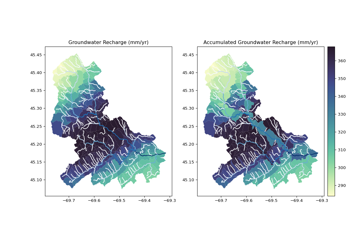
Python catchment characteristics accumulation
R client Application
First, we will retrieve some data and build a simple plot of our area of
interest using
plot_nhdplus()
from nhdplusTools
.
    library(dplyr)
    library(sf)
    library(nhdplusTools)

    nldi_feature <- list(featureSource = "nwissite",
                         featureID = "USGS-01031500")

    outlet_comid <- discover_nhdplus_id(nldi_feature = nldi_feature)

    data <- plot_nhdplus(nldi_feature, flowline_only = FALSE)
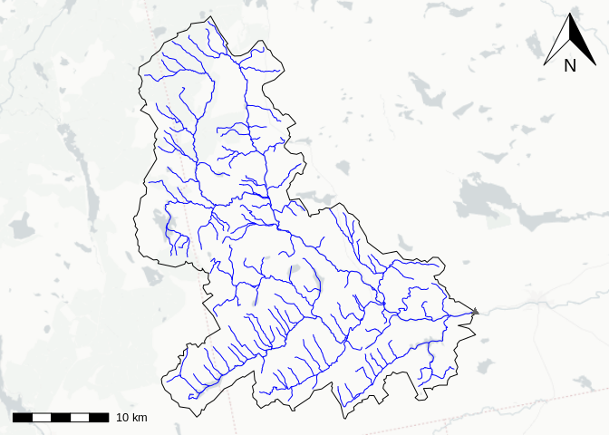
Preview map of watershed
Now we can use
discover_nldi_characteristics()
to find out what characteristics are available from the NLDI and get
them for the outlet of our area of interest with
get_nldi_characteristics()
    chars <- discover_nldi_characteristics()

    outlet_total <- get_nldi_characteristics(nldi_feature, type = "total")

    outlet_total <- left_join(outlet_total$total, chars$total,
                              by = "characteristic_id")

    outlet_total <- outlet_total %>%
      select(ID = characteristic_id,
                           Description = characteristic_description,
                           Value = characteristic_value,
                           Units = units,
                           link = dataset_url) %>%
      mutate(link = paste0('<a href="', link, '">link</a>'))

    knitr::kable(outlet_total)
| ID | Description | Value | Units | link |
|---|---|---|---|---|
| TOT_BFI | Base Flow Index (BFI), The BFI is a ratio of base flow to total streamflow, expressed as a percentage and ranging from 0 to 100. Base flow is the sustained, slowly varying component of streamflow, usually attributed to ground-water discharge to a stream. | 46 | percent | link |
| TOT_CONTACT | Subsurface flow contact time index. The subsurface contact time index estimates the number of days that infiltrated water resides in the saturated subsurface zone of the basin before discharging into the stream. | 137.57 | days | link |
| TOT_ET | Mean-annual actual evapotranspiration (ET), estimated using regression equation of Sanford and Selnick (2013) | 468 | mm/year | link |
| TOT_EWT | Average depth to water table relatice to the land surface(meters) | -21.62 | meters | link |
| TOT_HGA | Percentage of Hydrologic Group A soil. -9999 denotes NODATA, usually water. Hydrologic group A soils have high infiltration rates. Soils are deep and well drained and, typically, have high sand and gravel content. | 4.47 | percent | link |
| TOT_HGAC | Percentage of Hydrologic Group AC soil. -9999 denotes NODATA, usually water. Hydrologic group AC soils have group A characteristics (high infiltration rates) when artificially drained and have group C characteristics (slow infiltration rates) when not drained. | 0 | percent | link |
| TOT_HGAD | Percentage of Hydrologic Group AD soil. -9999 denotes NODATA, usually water. Hydrologic group AD soils have group A characteristics (high infiltration rates) when artificially drained and have group D characteristics (very slow infiltration rates) when not drained. | 0 | percent | link |
| TOT_HGB | Percentage of Hydrologic Group B soil. -9999 denotes NODATA, usually water. Hydrologic group B soils have moderate infiltration rates. Soils are moderately deep, moderately well drained, and moderately coarse in texture. | 14.2 | percent | link |
| TOT_HGBC | Percentage of Hydrologic Group BC soil. -9999 denotes NODATA, usually water. Hydrologic group BC soils have group B characteristics (moderate infiltration rates) when artificially drained and have group C characteristics (slow infiltration rates) when not drained. | 0 | percent | link |
| TOT_HGBD | Percentage of Hydrologic Group BD soil. -9999 denotes NODATA, usually water. Hydrologic group BD soils have group B characteristics (moderate infiltration rates) when artificially drained and have group D characteristics (very slow infiltration rates) when not drained. | 0 | percent | link |
| TOT_HGC | Percentage of Hydrologic Group C soil. -9999 denotes NODATA, usually water. Hydrologic group C soils have slow soil infiltration rates. The soil profiles include layers impeding downward movement of water and, typically, have moderately fine or fine texture. | 41.66 | percent | link |
| TOT_HGCD | Percentage of Hydrologic Group CD soil. -9999 denotes NODATA, usually water. Hydrologic group CD soils have group C characteristics (slow infiltration rates) when artificially drained and have group D characteristics (very slow infiltration rates) when not drained. | 16.84 | percent | link |
| TOT_HGD | Percentage of Hydrologic Group D soil. -9999 denotes NODATA, usually water. Hydrologic group D soils have very slow infiltration rates. Soils are clayey, have a high water table, or have a shallow impervious layer. | 22.83 | percent | link |
| TOT_HGVAR | Percentage of Hydrologic Group VAR soil. -9999 denotes NODATA, usually water. Hydrologic group VAR soils have variable drainage characteristics. | 0 | percent | link |
| TOT_IEOF | Percentage of Horton overland flow as a percent | 2.29 | percent | link |
| TOT_OLSON_PERM | Rock hydraulic conductivity (10^-6 m/s). | 0.12 | 10^-6 m/s | link |
| TOT_PEST219 | Estimate of agricultural pesticide application (219 types), kg/sq km, from Census of Ag 1997, based on county-wide sales and percent agricultural land cover in watershed | 2.32 | kg/sqkm | link |
| TOT_PET | Mean-annual potential evapotranspiration (PET), estimated using the Hamon (1961) equation. | 512.18 | mm/year | link |
| TOT_PPT7100_ANN | Mean annual precip (mm) for the watershed, from 800m PRISM data. 30 years period of record 1971-2000. | 1180.7 | mm/year | link |
| TOT_RECHG | Mean annual natural ground-water recharge in millimeters per year | 336.26 | mm/yr | link |
| TOT_RH | Watershed average relative humidity (percent), from 2km PRISM, derived from 30 years of record (1961-1990). | 68.48 | percent | link |
| TOT_ROCKTYPE_100 | Estimated percent of catchment that is underlain by the Principal Aquifer rock type, Unconsolidated sand and gravel aquifers. | 0 | percent | link |
| TOT_ROCKTYPE_200 | Estimated percent of catchment that is underlain by the Principal Aquifer rock type, Semiconsolidated sand aquifers. | 0 | percent | link |
| TOT_ROCKTYPE_300 | Estimated percent of catchment that is underlain by the Principal Aquifer rock type, Sandstone aquifers. | 0 | percent | link |
| TOT_ROCKTYPE_400 | Estimated percent of catchment that is underlain by the Principal Aquifer rock type, Carbonate-rock aquifers. | 0 | percent | link |
| TOT_ROCKTYPE_500 | Estimated percent of catchment that is underlain by the Principal Aquifer rock type, Sandstone and carbonate-rock aquifers. | 0 | percent | link |
| TOT_ROCKTYPE_600 | Estimated percent of catchment that is underlain by the Principal Aquifer rock type, Igneous and metamorphic-rock aquifers. | 0 | percent | link |
| TOT_ROCKTYPE_999 | Estimated percent of catchment that is underlain by the Principal Aquifer rock type, Other rocks. | 100 | percent | link |
| TOT_RUN7100 | Estimated 30-year (1971-2000) average annual runoff in millimeters per year | 738.61 | millimeters per year | link |
| TOT_SATOF | Percentage of Dunne overland flow as a percent | 3.3 | percent | link |
| TOT_TAV7100_ANN | Watershed average of monthly air temperature (degrees C) from 800m PRISM, derived from 30 years of record (1971-2000). | 4.13 | degrees C | link |
| TOT_TWI | Topographic wetness index, ln(a/S); where ln is the natural log, a is the upslope area per unit contour length and S is the slope at that point. See http://ks.water.usgs.gov/Kansas/pubs/reports/wrir.99-4242.html and Wolock and McCabe, 1995 for more detail | 11.55 | ln(m) | link |
| TOT_WB5100_ANN | unknown | 643.08 | unknown | link |
Now, for the sake of demonstration, we will run get_nldi_characteristics for all the catchments in our area of interest.
**NOTE: This will be slow for large collections of characteristics. For large collections, download the characteristics directly from the source.
    characteristic <- "CAT_RECHG"
    tot_char <- "TOT_RECHG"

    all_local <- sapply(data$flowline$COMID, function(x, char) {
      chars <- get_nldi_characteristics(
        list(featureSource = "comid", featureID = as.character(x)),
        type = "local")

      filter(chars$local, characteristic_id == char)$characteristic_value

    }, char = characteristic)

    local_characteristic <- data.frame(COMID = data$flowline$COMID)
    local_characteristic[[characteristic]] = as.numeric(all_local)

    cat <- right_join(data$catchment, local_characteristic, by = c("FEATUREID" = "COMID"))

    plot(cat[characteristic])
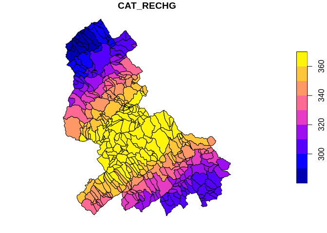
Plot of catchments with local characteristic values
Now that we have the local characteristics, we can run a downstream
accumulation with an internal nhdplusTools function
accumulate_downstream(). The plot at the bottom here shows the
accumulated characteristic and the output values at the bottom show that
we get the same answer from locally-calculated accumulation or the total
accumulated pre-calculated characteristic! So that’s good.
    net <- prepare_nhdplus(data$flowline, 0, 0, 0, purge_non_dendritic = FALSE, warn = FALSE)

    ## Warning in prepare_nhdplus(data$flowline, 0, 0, 0, purge_non_dendritic =
    ## FALSE, : Got NHDPlus data without a Terminal catchment. Attempting to find it.

    net <- select(net, ID = COMID, toID = toCOMID) %>%
      left_join(select(st_drop_geometry(data$flowline), COMID, AreaSqKM),
                by = c("ID" = "COMID")) %>%
      left_join(local_characteristic, by = c("ID" = "COMID"))


    net[["temp_col"]] <- net[[characteristic]] * net$AreaSqKM

    net[[tot_char]] <- nhdplusTools:::accumulate_downstream(net, "temp_col")
    net$DenTotDASqKM <- nhdplusTools:::accumulate_downstream(net, "AreaSqKM")

    net[[tot_char]] <- net[[tot_char]] / net$DenTotDASqKM

    cat <- right_join(data$catchment,
                      select(net, -temp_col, -toID, -DenTotDASqKM),
                      by = c("FEATUREID" = "ID"))

    plot(cat[tot_char], reset = FALSE)
    plot(st_geometry(data$flowline), add = TRUE, lwd = data$flowline$StreamOrde, col = "lightblue")
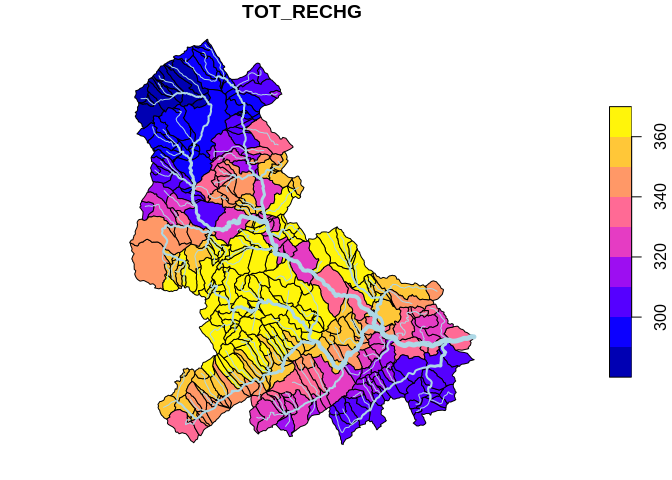
Plot of accumulated characteristic
    filter(outlet_total, ID == tot_char)$Value

    ## [1] "336.26"

    filter(cat, FEATUREID == outlet_comid)[[tot_char]]

    ## [1] 336.2556
They match! So that’s good.
Categories:
Related Posts
The Hydro Network-Linked Data Index
November 2, 2020
Introduction
updated 11-2-2020 after updates described here .
updated 9-20-2024 when the NLDI moved from labs.waterdata.usgs.gov to api.water.usgs.gov/nldi/
The Hydro Network-Linked Data Index (NLDI) is a system that can index data to NHDPlus V2 catchments and offers a search service to discover indexed information. Data linked to the NLDI includes active NWIS stream gages , water quality portal sites , and outlets of HUC12 watersheds . The NLDI is a core product of the Internet of Water and is being developed as an open source project. .
The Network Linked Data Index (NLDI) Geoprocessing with OGC API Processes
April 12, 2022
The Network Linked Data Index (NLDI) is a search engine that indexes data to the flowpaths and/or catchments of a river network and provides discovery services based on position in that network. Like a search engine, it can cache and index new data. It also offers some convenient data services like basin boundaries and accumulated catchment characteristics.
Cloud-optimized USGS time series data
January 8, 2020
Intro
The scalability, flexibility, and configurabilty of the commercial cloud provide new and exciting possibilities for many applications including earth science research. As with many organizations, the US Geological Survey (USGS) is exploring the use and advantages of the cloud for performing their science. The full benefit of the cloud, however, can only be realized if the data that will be used is in a cloud-friendly format.
Additional field measurements are coming to WDFN
June 25, 2026
Water Data for the Nation (WDFN) publishes multiple categories of data collected at our monitoring locations, including both data collected by automated sensors and through manual methods. Manually collected data, which we refer to as “field measurements,” are collected during visits to a monitoring location.
What's new with WDFN APIs - Summer 2026 Edition
June 18, 2026
It’s been a busy few months for Water Data for the Nation’s Water Data APIs , the services that publish USGS water data in machine-readable formats. This post walks through a few recent updates to these APIs.