Reproducible Data Science in R: Flexible functions using tidy evaluation
Improve your functions with helpful dataframe evaluation patterns.
What's on this page

Overview
This blog post is part of a series that works up from functional programming foundations through the use of the targets R package to create efficient, reproducible data workflows.
Where we're going: This article addresses the common challenges associated with writing flexible data wrangling functions that leverage the tidyverse ecosystem for dataframe operations. It will first introduce the quirks and patterns of tidy evaluation before covering an example that utilizes techniques such as data masking and tidy selection to support function flexibility. By the end of the blog, the reader will be familiar with tidy evaluation patterns useful for writing functions. This post may also serve as a reference for R programmers looking for a reminder on these techniques.
Audience: This article assumes some familiarity with writing functions in R and using common dplyr functions.
Function flexibility challenges
In code development, choosing the ideal level of input flexibility for a custom-written function is a non-trivial decision. While flexible functions are often broadly applicable across coding projects (yay reusability!), they require more up front prep work to ensure specifications are clearly documented AND there’s consistency in the code’s functionality across the range of allowable inputs.
In particular, combining function input flexibility with the tidyverse ecosystem often requires adding some new pieces of syntax to the mix: for instance, have you noticed that dplyr functions don’t require you to add quotation marks around variable names? This is generally a very handy feature that saves time and keystrokes. However, when these functions are within custom functions that you write, they require some special handling. Why? Because in an attempt to make tidyverse functions efficient to use, the developers tweaked the way the functions evaluate inputs, straying away from the standard evaluation methods used by R. This form of non-standard evaluation is termed (surprise 🥳!) tidy evaluation.
Have you seen syntax like {{ }}, !!, .data[[ ]], or quo()/enquo() before? These are all examples of methods to alter evaluation contexts in R, which are particularly helpful while building your own flexible functions that leverage the tidyverse to seamlessly perform:
- dynamic variable selection
- grouped variable operations
- plot parameterization
Evaluation in R
In the context of tidy evaluation, it bears reiterating (from previous blog posts
) that environments play a role in the process of evaluating code in R. When you open up an R session, any objects you define (including functions) will be added to the global environment. Functions you have authored also have their own unique environments created and destroyed every time you run them. If you introduce something into your function that isn’t explicitly defined in the function or its inputs, like x in the following function, add_stuff:
x <- 5

add_stuff <- function(y){
  z <- x + y
  return(z)
}

add_stuff(y = 10)
#> [1] 15
…R will look for x in the add_stuff function environment first, but it’s not there (the only input is y)! It will then look into the function’s enclosing environment, which in this case is the global environment, locate the expression x <- 5, and use that in its evaluation of z <- x + y.
Functions in the tidyverse excel at modifying evaluation in an attempt to improve the user experience. Let’s take a look at a base R and tidyverse approach to the same operation. In the example below, we are selecting two columns from the palmerpenguins
dataset by name:
library(palmerpenguins)
library(dplyr)

# base R
base_selection <- penguins[,c("species", "island")]

# dplyr
dplyr_selection <- select(penguins, species, island)
Notice how in base R, we select columns using a vector of strings in quotation marks, but using dplyr::select(), we don’t need to use quotation marks to denote column names. This tidyverse implementation strays from the usual evaluation methods in R, because the normal base R method would look for objects called species and island throughout all enclosing environments, turn up empty handed, and throw an error. The tidyverse’s “slight of hand” under the hood sometimes delays evaluation of an input, or searches for an expression in a way that does not match R’s out-of-the-box methods for evaluation.
In the above example, you can think of dplyr invisibly adding quotation marks to the arguments in select() before evaluating them and recognizes the inputs to select() as columns in the penguins dataframe. This is called data masking and is the result of dplyr essentially attaching the dataframe as its most immediate environment to search for data variables (like column names). Note that data variables are specific to the dataframe and are distinct from environment variables, which are present in the global environment and other enclosing environments (e.g. the dataframe penguins is an environment variable). The following dplyr functions utilize data masking:
arrange()count()filter()group_by()mutate()summarise()
Another prominent tidy evaluation method is called tidy selection, which leverages a useful set of modifiers like all_of(), any_of(), starts_with(), and where() to determine which columns a dplyr function will use. The following dplyr functions utilize tidy selection (sometimes in addition to data masking):
across()relocate()rename()select()pull()
Tidy evaluation patterns
The following expandable sections cover the most common tidy evaluation techniques and use cases. Click on each heading to learn more about when and how to use each technique. Next, we will use a real-world data analysis scenario to go into more detail on each technique.
.data[[ ]] pronoun
Category: Data masking
Input format within
function(): column_name = "Column_A"When to use: Your function uses
tidyverse functions on column name inputs denoted by strings. Note that in most cases, you cannot use .data[[ ]] on the left-hand side of an operation (i.e. to the left of an = assignment). There's a bit of a funky reason for this that has to do with the fact that .data[[ ]] doesn't actually represent a dataframe; instead it is a construct used to grab data variables in the context of the dataframe being evaluated (here's a great discussion about it on the Posit forum). In other words, it's more or less a "stand-in" for referencing elements of a dataframe.If you want to perform an operation (using something like
mutate()) on a column you'd normally pass to the .data[[ ]] pronoun, you usually have to use the curly-curly braces on the left-hand side:{{ }}. Check out the next expandable section for more information on curly-curly.Caveat: you can use
.data[[ ]] on the left-hand side of a filtering function, like this: filter(.data[[column_name]] == .data[["Column_B"]]). Tricky.Example structure:
mutate(new_column = .data[[ column_name ]] * 2)curly-curly (a.k.a. embrace) {{ }} and injection :=
Category: Data masking
Input format within
function(): column_name = Column_A; column_name = "Column_A"When to use: Your function uses
tidyverse functions on variable column name inputs, and the .data[[ ]] pronoun won't work. If your function accepts column names without quotation marks, you can use {{ }} on both the left and right sides of an operation, like within mutate(). If your function accepts column names with quotation marks, you can only use {{ }} on the left-hand side of the operation. The use of curly-curly is a recent addition to the tidy evaluation suite, replacing most uses of !! (bang bang) and quo()/enquo(). Check out this section of Stanford's Data Challenge Lab course for an excellent explanation of curly-curly's predecessor, the !!enquo() pattern.Example structure(s):
mutate({{ column_name }} := {{ column_name }} * 2)mutate({{ column_name }} := .data[[ column_name ]] * 2)all_of() and any_of()
Category: Tidy selection
Input format within
function(): column_names = c("Column_A", "Column_B")When to use: Your function performs
tidyverse operations on more than one input column at a time and those column names have quotation marks.Example structure:
select(all_of(column_names))across()
Category: Both
Input format within
function(): column_names = c("Column_A", "Column_B")When to use: You want to pass multiple column names with quotation marks to a function that uses data masking.
Example structure:
group_by(across(all_of(column_names)))"{ }_name" :=
Category: Data masking
Input format within
function():column_name = "Column_A"When to use: You want to use a column name input to name a new column produced by your function (using
tidyverse operations) and the column name is in quotation marks. Note that this trick leverages the glue package to paste together inputs and character strings, and elsewhere you may need to call glue() specifically to include this functionality.Example structure:
mutate("{ column_name }_timestwo" := .data[[ column_name ]] * 2)"{{ }}_name" :=
Category: Data masking
Input format within
function():column_name = Column_AWhen to use: You want to use a column name input to name a new column produced by your function (using
tidyverse operations) and the column name is not in quotation marks. Note that this trick leverages the glue package to paste together inputs and character strings, and elsewhere you may need to call glue() specifically to include this functionality (see data analysis workflow in next section for an example using the glue package).Example structure:
mutate("{{ column_name }}_timestwo" := {{ column_name }} * 2)ellipsis ...
Category: Data masking
Input format within
function():Column_A, Column_BWhen to use: You want to pass a list of column name inputs without quotation marks directly into a
tidyverse function or set of functions.Example structure:
group_by(...) or select(...)Going deeper: an example workflow
Now that we have a better understanding of tidy evaluation and the patterns for working with it, let’s examine a scenario currently pertinent to users of Water Quality Portal (WQP)
data. In 2024, the WQP team initiated a transition to the new WQX3.0 format
from the WQX version 2 format (we will refer to it as “legacy”). While still under development, this switch includes changes to the field names (and in some cases, field values) returned from the database. NOTE that as of March 2024 newly uploaded or corrected USGS data are not available in the legacy data format. The dataRetrieval team has created an informative status page
on this transition, complete with examples of WQX3.0 and legacy data pulls.
This scenario is a great opportunity to develop a function that leverages tidy evaluation in a way that it is flexible to both the legacy and WQX3.0 formats. Say we had already written a script that downloads data in the legacy format from the WQP from a single site and plots the most sampled water chemistry constituents (reported in micrograms per liter, ug/L) using an interactive ggplotly plot. We’ll use the Kawishiwi River outside of Ely, MN as our example site. Our legacy dataset might look something like this, using the most recent development version of dataRetrieval :
# Load required packages
# Install using install.packages() if you don't have them.
# Version numbers used provided in comments
library(dataRetrieval) # 2.7.17.9000, from GitHub
library(dplyr) # 1.1.4
library(lubridate) # 1.9.4
library(plotly) # 4.10.0
library(khroma) # 1.14.0, colorblind-accessible color palettes
library(glue) # 1.8.0
library(rlang) # 1.1.4

# Download legacy data
kawishiwi <- dataRetrieval::readWQPdata(
  siteid = 'USGS-05124480',
  service = 'Result'
)

# Take a look at what we're working with
kawishiwi |>
  dplyr::arrange(ActivityStartDate, CharacteristicName) |>
  dplyr::select(ActivityStartDate, CharacteristicName,
                ResultMeasureValue, ResultMeasure.MeasureUnitCode) |>
  head()

#>   ActivityStartDate CharacteristicName ResultMeasureValue ResultMeasure.MeasureUnitCode
#> 1        1966-07-21      Acidity, (H+)            0.00013                          mg/l
#> 2        1966-07-21         Alkalinity                 11                    mg/l CaCO3
#> 3        1966-07-21           Altitude               1450                            ft
#> 4        1966-07-21           Aluminum                400                          ug/l
#> 5        1966-07-21        Bicarbonate                 13                          mg/l
#> 6        1966-07-21              Boron                 30                          ug/l
Our original script and plot output might look something like this (click to view code and plot):
# Make timeseries plot of WQ data

min_years <- 10

common_constituents <- kawishiwi |>
  # select columns used
  dplyr::select(ResultMeasure.MeasureUnitCode, ResultMeasureValue,
                ActivityStartDate, CharacteristicName) |>
  # filter to micrograms per liter
  dplyr::filter(ResultMeasure.MeasureUnitCode %in% c("ug/l", "ug/L")) |>
  # ensure result value is numeric,
  # convert character string of dates to dates,
  # and grab year for filtering later
  dplyr::mutate(
    ResultMeasureValue_numeric = as.numeric(ResultMeasureValue),
    ActivityStartDate = as.Date(ActivityStartDate, "%y-%m-%d"),
    year = lubridate::year(ActivityStartDate)
  ) |>
  # get rid of NAs
  dplyr::filter(!is.na(ResultMeasureValue_numeric)) |>
  # arrange dataset by date
  dplyr::arrange(ActivityStartDate) |>
  # count the number of years of data collected
  # per characteristic, and then filter to
  # characteristics with at least n years of data
  dplyr::group_by(CharacteristicName) |>
  dplyr::mutate(n_years = length(unique(year))) |>
  dplyr::filter(n_years >= min_years) |>
  dplyr::ungroup()

# use ggplot to create a timeseries plot
p <- ggplot2::ggplot(data = common_constituents,
                     ggplot2::aes(x = ActivityStartDate,
                         y = ResultMeasureValue_numeric,
                         color = CharacteristicName)) +
  ggplot2::geom_line() +
  ggplot2::geom_point() +
  ggplot2::labs(x = "Date",
                y = "Concentration (ug/l)",
                color = "Characteristic Name") +
  ggplot2::theme_minimal() +
  khroma::scale_color_vibrant()

# Make it an interactive plot (plot is not interactive in this blog)!
plotly::ggplotly(p)
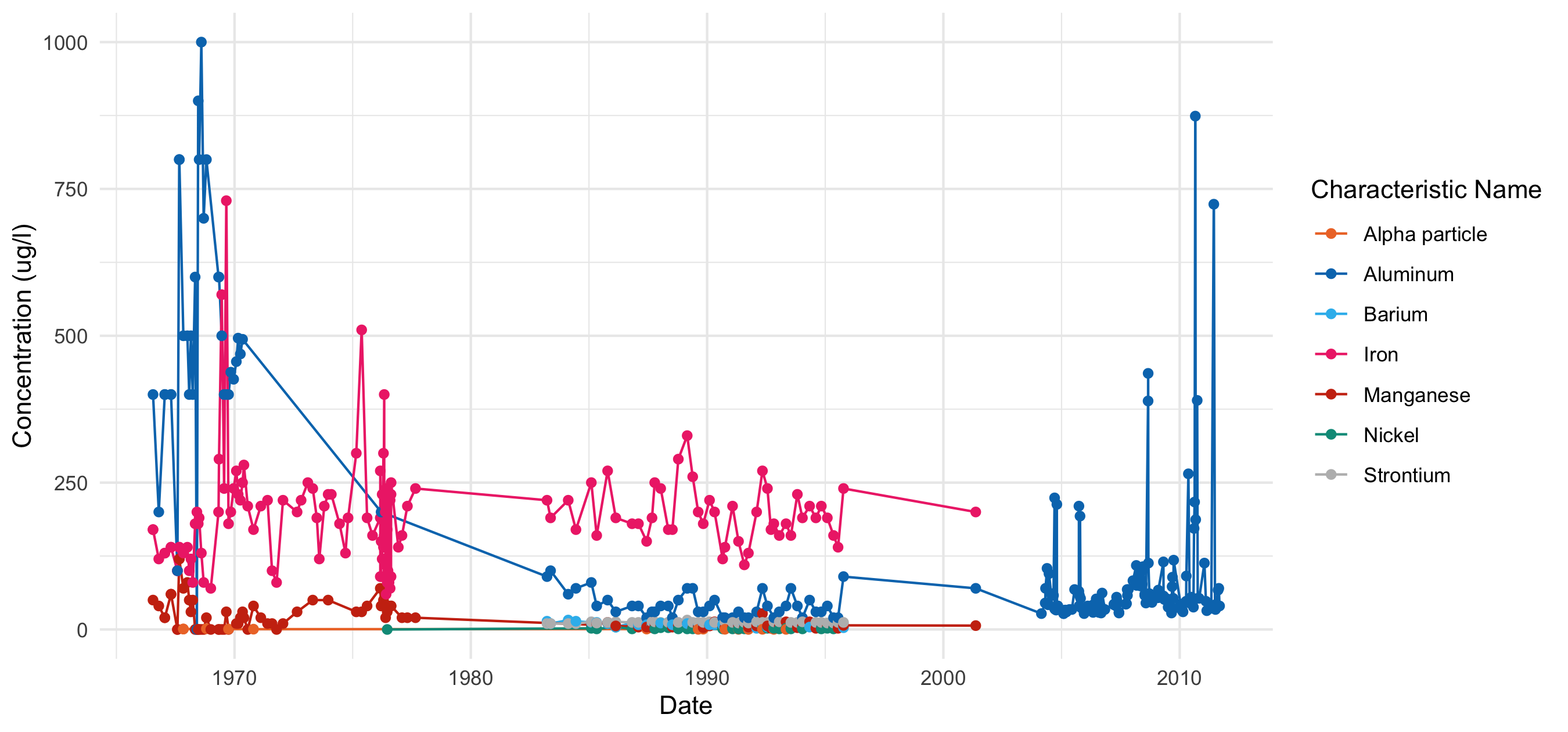
Timeseries scatterplot of constituents with at least 10 years of data on the Kawishiwi River, downloaded using the legacy WQP database.
Next, let’s download the same dataset in the WQX3.0 format and take a look at its new structure:
# Download the WQX3.0 version data
kawishiwi_3.0 <- dataRetrieval::readWQPdata(
  siteid = 'USGS-05124480',
  service = 'ResultWQX3',
  dataProfile = 'fullPhysChem'
)

kawishiwi_3.0 |>
  dplyr::arrange(Activity_StartDate, Result_Characteristic) |>
  dplyr::select(Activity_StartDate, Result_Characteristic, Result_Measure, Result_MeasureUnit) |>
  head()

#>   Activity_StartDate Result_Characteristic Result_Measure Result_MeasureUnit
#> 1         1966-07-21         Acidity, (H+)        0.00013               mg/L
#> 2         1966-07-21            Alkalinity             11               mg/L
#> 3         1966-07-21              Altitude           1450                 ft
#> 4         1966-07-21              Aluminum            400               ug/L
#> 5         1966-07-21           Bicarbonate             13               mg/L
#> 6         1966-07-21                 Boron             30               ug/L
The challenge: As we suspected, the column names differ between the two WQX formats (e.g. ActivityStartDate versus Activity_StartDate), among other slight discrepancies (ug/"l" versus ug/"L" units). It would be a bit tedious and error-prone to copy, paste, and adapt the code above to our new dataset. And then what if another similar dataset comes along in the future?
The solution(s):With a little bit of forethought, we can tackle these dataframe variability challenges by writing a function that accepts the column names as inputs and leverages some tidy evaluation tricks. We will show you two solutions to generalizing the script into a function: one that uses quotation marks around the inputs, and one that does not.
Option 1: Use quotation marks around function inputs
The function below expects the column name inputs to have quotation marks around them, and leverages .data[[ ]] liberally. The function documentation is clear on this detail. Also notice that we build the new column name "{ result_column }_numeric" by pasting strings together using the glue() function from the glue
package. glue() is helpful because it evaluates expressions in curly brackets and pastes the result into an input string:
#' Make timeseries plot of WQ data
#'
#' @param wqp_dataframe A dataframe containing water quality data.
#' @param unit_column A character string in quotation marks matching the name
#'  of the unit column in`wqp_dataframe`.
#' @param date_column A character string in quotation marks matching the name
#'  of the date column in `wqp_dataframe`. Expects the date column to be data
#'  type character in the format "YYYY-MM-DD".
#' @param result_column A character string in quotation marks matching the name
#'  of the result value column in `wqp_dataframe`. Expects the result value
#'  column to be data type numeric.
#' @param grouping_column A character string in quotation marks matching the
#'  name of the column being used to group the data in `wqp_dataframe`.
#' @param min_years Numeric. A single number indicating the minimum number of
#'  years of data collected.
#'
#' @return A plotly plot showing water quality constituent concentrations for
#'  which min_years or more years of data have been collected.
#'

plot_timeseries <- function(wqp_dataframe,
                            unit_column,
                            date_column,
                            result_column,
                            grouping_column,
                            min_years) {

  plot_dataframe <- wqp_dataframe |>
    dplyr::select(all_of(c(unit_column, date_column, result_column, grouping_column))) |>
    dplyr::mutate({{ unit_column }} := tolower(.data[[unit_column]])) |>
    # filter to micrograms per liter
    dplyr::filter(.data[[unit_column]] == "ug/l") |>
    # ensure result value is numeric,
    # convert character string of dates to dates,
    # and grab year for filtering later
    dplyr::mutate(
      "{ result_column }_numeric" := as.numeric(.data[[result_column]]),
      {{ date_column }} := as.Date(.data[[date_column]], "%y-%m-%d"),
      year = lubridate::year(.data[[date_column]])
    ) |>
    # get rid of NAs
    dplyr::filter(!is.na(.data[[glue::glue("{ result_column }_numeric")]])) |>
    # arrange dataset by date
    dplyr::arrange(.data[[date_column]]) |>
    # count the number of years of data collected
    # per characteristic, and then filter to
    # characteristics with at least n years of data
    dplyr::group_by(.data[[grouping_column]]) |>
    dplyr::mutate(n_years = length(unique(year))) |>
    dplyr::filter(n_years >= min_years) |>
    dplyr::ungroup()

  # use ggplot to create a timeseries plot
  p <- ggplot2::ggplot(data = plot_dataframe, ggplot2::aes(
    x = .data[[date_column]],
    y = .data[[glue::glue("{ result_column }_numeric")]],
    color = .data[[grouping_column]])) +
    ggplot2::geom_line() +
    ggplot2::geom_point() +
    ggplot2::labs(x = "Date", y = "Concentration (ug/l)") +
    ggplot2::theme_minimal() +
    khroma::scale_color_muted()

  # Make it an interactive plot (plot is not interactive in this blog)!
  pi <- plotly::ggplotly(p)

  return(pi)
}
Let’s give this function a go with our new Kawishiwi River dataset from WQX3.0.
# Plot WQX3.0 dataset
plot_timeseries(
  wqp_dataframe = kawishiwi_3.0,
  unit_column = "Result_MeasureUnit",
  date_column = "Activity_StartDate",
  result_column = "Result_Measure",
  grouping_column = "Result_Characteristic",
  min_years = 10
)
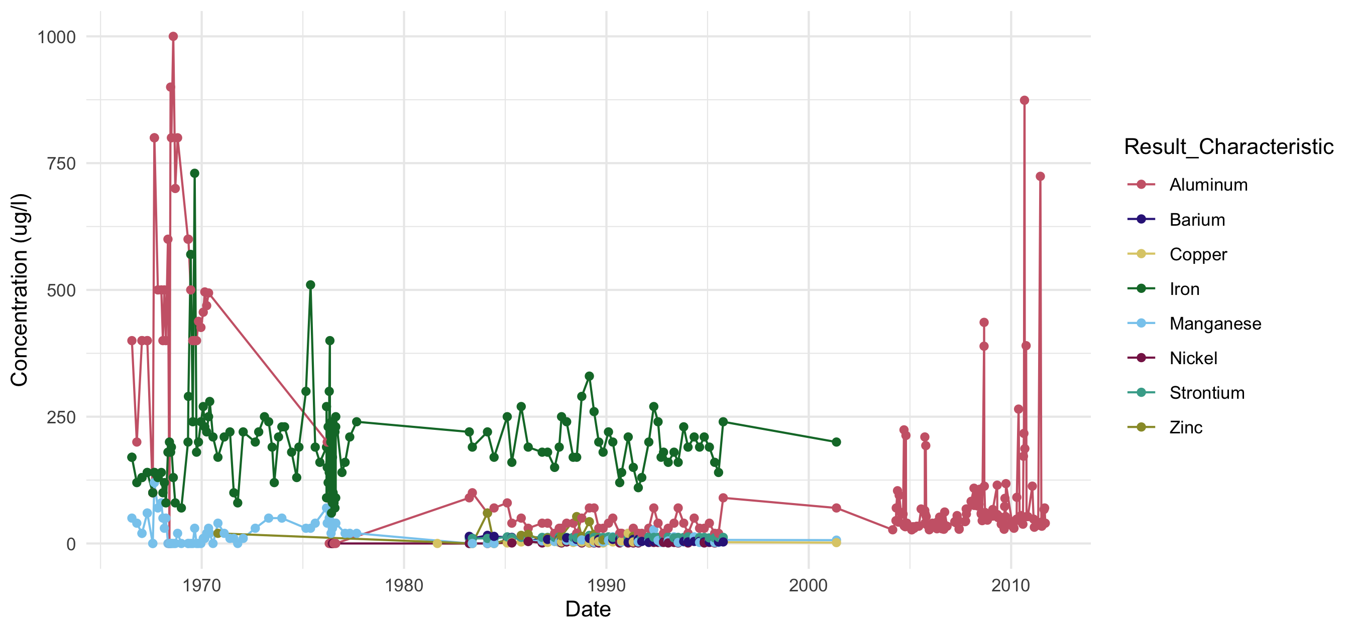
Timeseries scatterplot of constituents with at least 10 years of data on the Kawishiwi River, downloaded using the WQX 3.0 database.
Option 2: No quotation marks around function inputs
First, we define the new column name that will hold numeric result values. In order to make this column play nice with the rest, though, we first need to "defuse" the
result_column input to an expression using rlang::enquo() and then convert that expression to a string using rlang::as_label(). Once the result column name is categorized as a string, it can then be pasted to the additional text used to describe the new column (_numeric in the example below). This results in a string in quotation marks that is then converted to a symbol that the tidyverse functions can understand in the context of the dataframe being evaluated.The function below expects the column name inputs without quotation marks around them, and leverages {{ }} := {{ }} along with some rlang metaprogramming functions
for column name genesis:
#' Make timeseries plot of WQ data
#'
#' @param wqp_dataframe A dataframe containing water quality data.
#' @param unit_column A character string matching the name of the unit column
#'  in `wqp_dataframe`.
#' @param date_column A character string matching the name of the date column
#'  in `wqp_dataframe`. Expects the date column to be data type character in
#'  theformat "YYYY-MM-DD".
#' @param result_column A character string matching the name of the result
#'  value column in `wqp_dataframe`. Expects the result value column to be
#'  data type numeric.
#' @param grouping_column A character string matching the name of the column
#'  being used to group the data in `wqp_dataframe`.
#' @param min_years Numeric. A single number indicating the minimum number of
#'  years of data collected.
#'
#' @return A plotly plot showing water quality constituent concentrations for
#'  which min_years or more years of data have been collected.
#'

plot_timeseries <- function(wqp_dataframe,
                            unit_column,
                            date_column,
                            result_column,
                            grouping_column,
                            min_years) {

  # create new column name for column that will hold numeric version
  # of result_column. First, we'll "defuse" the input column name by
  # wrapping it in enquo(), then convert it to a string-like object
  # so it can be pasted together with "_numeric". Lastly, we use sym
  # to convert it to a symbol, much like all of the other input column
  # names.
  numeric_result_column <- rlang::sym(
    paste0(rlang::as_label(rlang::enquo(result_column)), "_numeric")
    )

  plot_dataframe <- wqp_dataframe |>
    dplyr::select({{ unit_column }}, {{ date_column }},
                  {{ result_column }}, {{ grouping_column }}) |>
    dplyr::mutate({{ unit_column }} := tolower({{ unit_column }})) |>
    # filter to micrograms per liter
    dplyr::filter({{ unit_column }} == "ug/l") |>
    # ensure result value is numeric,
    # convert character string of dates to dates,
    # and grab year for filtering later
    dplyr::mutate(
      {{ numeric_result_column }} := as.numeric({{ result_column }}),
      {{ date_column }} := lubridate::ymd({{ date_column }}),
      year = lubridate::year({{ date_column }})
    ) |>
    # get rid of NAs
    dplyr::filter(!is.na({{ numeric_result_column }})) |>
    # arrange dataset by date
    dplyr::arrange({{ date_column }}) |>
    # count the number of years of data collected
    # per characteristic, and then filter to
    # characteristics with at least n years of data
    dplyr::group_by({{ grouping_column }}) |>
    dplyr::mutate(n_years = length(unique(year))) |>
    dplyr::filter(n_years >= min_years) |>
    dplyr::ungroup()

  # use plotly to plot all characteristics on same plot
  p <- ggplot2::ggplot(data = plot_dataframe, ggplot2::aes(
    x = {{ date_column }},
    y = {{ numeric_result_column }},
    color = {{ grouping_column }})) +
    ggplot2::geom_line() +
    ggplot2::geom_point() +
    ggplot2::labs(x = "Date", y = "Concentration (ug/l)") +
    ggplot2::theme_minimal() +
    khroma::scale_color_muted()

  # Make it an interactive plot (plot is not interactive in this blog)!
  pi <- plotly::ggplotly(p)

  return(pi)
}
For fun, let’s try making a slightly different timeseries plot for kawishiwi_3.0, using characteristic group rather than characteristic name to visualize water quality through time:
plot_timeseries(
  wqp_dataframe = kawishiwi_3.0,
  unit_column = Result_MeasureUnit,
  date_column = Activity_StartDate,
  result_column = Result_Measure,
  grouping_column = Result_CharacteristicGroup,
  min_years = 10
)
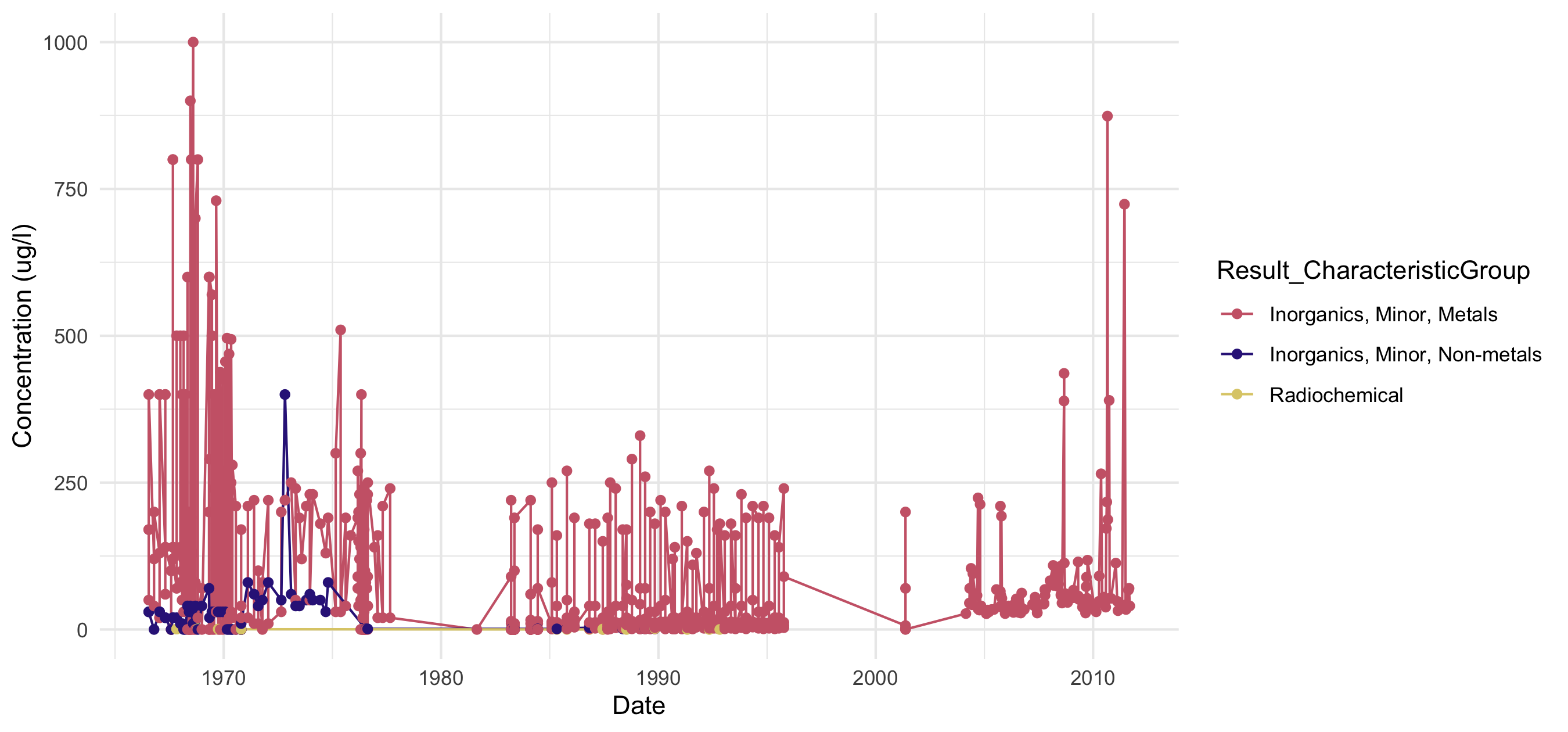
Timeseries scatterplot of constituent groups on the Kawishiwi River, downloaded using the WQX 3.0 database.
Well, would you look at that flexibility? 😎
Hopefully by now you’ve started gaining familiarity with tidy evaluation and feel inspired to give it a try in some of your upcoming analyses. This blog post only scratches the surface, and there is so much more to learn on this topic. If you want to dig deeper, check out the resources below, several of which go into the nitty gritty details of code evaluation.
Helpful resources
Quick tip: writing a package you want to submit to CRAN? Here's something to consider (click to expand)
Tidy evaluation uses syntax like
:= and .data, which fundamentally belong to the rlang package and are part of the suite of metaprogramming symbols/notations. If these symbols are not explicity imported from rlang in your package in the roxygen skeleton (ex. @importFrom rlang :=) and rlang is not added as an Import in the DESCRIPTION file, it can lead to issues with R CMD check/devtools::check throwing the note: no visible binding for global variable [insert symbol here]. Additionally, tidyverse's data variables construct can lead R CMD check to throw the "no visible binding" note because it confuses data variables for undefined global objects. One way to avoid this is to define your data variables as global variables using utils::globalVariables("[var1]", "[var2]"). Check out this Posit forum for information on importing rlang syntax into your package and this Posit forum for information regarding data variables in an R package.Links to some additional reading on tidy evaluation:
References
DeCicco, L.A., Hirsch, R.M., Lorenz, D., Watkins, W.D., Johnson, M., 2024, dataRetrieval: R packages for discovering and retrieving water data available from Federal hydrologic web services, v.2.7.15, doi:10.5066/P9X4L3GE
Categories:
Related Posts
Reproducible Data Science in R: Iterate, don't duplicate
July 18, 2024

Overview
This blog post is part of a series that works up from functional programming foundations through the use of the targets R package to create efficient, reproducible data workflows.
Reproducible Data Science in R: Writing better functions
June 17, 2024

Overview
This blog post is part of a series that works up from functional programming foundations through the use of the targets R package to create efficient, reproducible data workflows.
Reproducible Data Science in R: Writing functions that work for you
May 14, 2024

Overview
This blog post is part of a series that works up from functional programming foundations through the use of the targets R package to create efficient, reproducible data workflows.
Reproducible Data Science in R: Say the quiet part out loud with assertion tests
September 2, 2025

Overview
This blog post is part of the Reprodicuble data science in R series that works up from functional programming foundations through the use of the targets R package to create efficient, reproducible data workflows.
A map that glows with the vocabulary of water
February 27, 2026
English is the official language and authoritative version of all federal information.
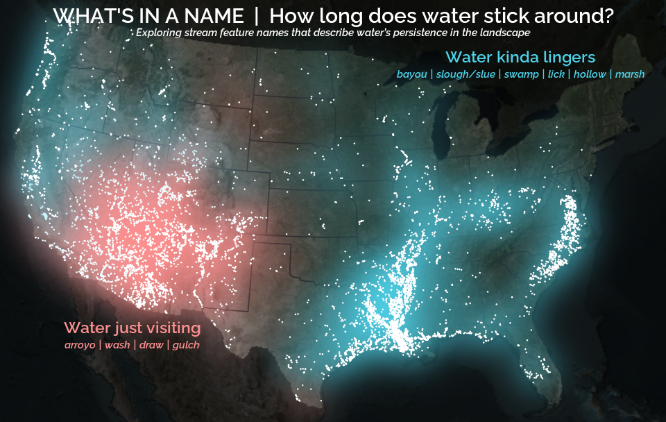
A map that glows with the vocabulary of water
What is your first impression of the map above? To me, it is the shimmer. Thousands of points of light, each one a stream or river, illuminating a darkened basemap. Look closely and a pattern emerges: the country’s waterways form a linguistic constellation. These points are classified not from population data or even explicitly by hydrology. They glow strictly according to the vocabulary used to name them and what can be implied about the hydrology of these streams based on their names.

