
Reproducible Data Science in R: Writing functions that work for you
Learn the ropes building your own functions in R using water data examples.
What's on this page
Overview
This blog post is part of a series that works up from functional programming foundations through the use of the targets R package to create efficient, reproducible data workflows.
Where we're going: This article covers writing your own functions in R, with a focus on water data. We will first go through the necessary elements of a function and briefly talk about environments in R. Then, we will work through a simple example of processing and summarizing data from the Water Quality Portal using a couple of approaches. By the end of this article, you should have the foundations needed to write custom functions: stay tuned for the next article in the series that covers leveling up your functions in R!
Audience: this article starts from a novice understanding of programming – this isn’t your first time opening up R or RStudio, but you’re still learning the ropes (let’s face it, we all are!).
Author's perspective: overcoming a fear of code (click here to expand)
Author's background (Elise): My first exposure to the R programming language was over 10 years ago in an undergraduate course, and it was 100% a shock to the system. I had never failed so hard to understand a new concept, and the steep learning curve felt like it was covered in ice: whatever progress I made was quickly reversed by an error that sent my confidence sliding down to the bottom (does this resonate with you?). It can be hard to pick yourself up to try to understand the miscommunication at hand...with a machine, no less. What's more, even searching for help can be a challenge---when you're a newer programmer, it's difficult to communicate through a web search what you're trying to get help with! But really, to me learning R and programming is an exercise in patience and connection more than anything else: the understanding will come...through talking with peers, slowing down, staying curious, and even sleeping on it.What is a custom function, why would I need one, and how do I make one?
The what: Functions belong to a class of objects that perform some action when called. They are recognizable by their name, followed by enclosing parentheses. If you program in R, you use functions everywhere, from read.csv() to sum() to mutate()
. While these functions are defined in base R or the source code of their respective packages, we can also write and use our own.
The why: Have you ever found yourself copying and pasting the same code chunk over and over in a script, perhaps changing one or two things about it with every iteration? While this may seem like an easy solution in the moment, it can become a liability later on when you need to make edits or an error inevitably crops up. Instead, a better approach might be to write a custom function you can invoke as many times as necessary in the script, where the inputs to the function are the things you frequently swapped out in your copy-paste routine. Writing functions improves consistency, portability, and reproducibility, reduces the chances of introducing errors, improves your ability to locate errors, and often saves many lines in your code (check out the don’t repeat yourself principle of software development for even more justification).
The how: Let’s take a look at a simple function that converts cubic feet per second (cfs) to cubic meters per second (cms).
# This function converts streamflow units from cubic feet per second (cfs) to
# cubic meters per second (cms) using a conversion constant
# https://www.convertunits.com/from/cubic%20feet%20per%20second/to/cubic%20meter%20per%20second.
# x must be a numeric value or vector

cfs_to_cms <- function(x){
  y <- x * 0.028316847
}
The function has three main components:
A name:
cfs_to_cmsA set of arguments. In this case, it is one argument,
x, which appears in the formatfunction(arguments)A body, enclosed by
{ }
The function will take the input argument, represented by x and run it through the equation in the body of the function to produce the output y. Because y is the last object in the body of the function, the function cfs_to_cms() will return whatever y is as the output. You could also write return(y) at the end of the function to explicitly define the output, like this:
# This function converts streamflow units from cubic feet per second (cfs) to
# cubic meters per second (cms) using a conversion constant
# https://www.convertunits.com/from/cubic%20feet%20per%20second/to/cubic%20meter%20per%20second.
# x must be a numeric value or vector

cfs_to_cms <- function(x){
  y <- x * 0.028316847

  return(y)
}
A primer on environments in R
In a script, every line generally performs some operation on an object, be it a number, string, vector, dataframe, list, etc. But where does this happen in the R programming space? Each of these operations (functions) is carried out within a specific environment in your R session. At its simplest, an environment is a list of named objects (vectors, dataframes, functions, other environments…) in no particular order that share space (or in R-speak: “bindings”) with one another.
We won’t get into the minutiae about environments, but it is important to recognize that by default, your R console opens up to the global environment. When you assign objects in the R console using <-, you are binding those objects to the global environment. Functions are neat in that they create their own environments: think about the body of the function { } as its own workspace where things happen, separate from the global environment. The function’s output, however, is still assigned to the global environment.
Why does this matter for our purposes? Well, just remember that objects defined in a function exist within the function’s environment and are isolated from the global environment (but see here ) unless they are returned from the function.
It is helpful to maintain separate function environments to avoid naming conflicts and isolate custom settings in each environment: how many functions in the R universe have objects in the function body named “data_summary” or “output”? Probably quite a few! Maintaining separate environments ensures those wires don’t get crossed if you happen to be using multiple functions with the same object names in their environments.
Running a custom function
To use the cfs_to_cms() function, you must first “run” the code chunk in the console to add it to the global environment, just like a line of code in a script. After that, we can start using the function on data! Let’s start by converting 100 cfs to cms:
# function output is not assigned to an object
cfs_to_cms(100)
#> [1] 2.831685
# function output assigned to an object named "flow"
flow <- cfs_to_cms(100)
flow
#> [1] 2.831685
According to our custom function, a flow of 100 cfs is equivalent to 2.83 cms. When cfs_to_cms(100) is not assigned to an object, its returned result (the object y inside the function) is simply printed in the console. However, we can assign that result to an object name, like flow, and it will be stored in the global environment. By typing flow into the R console, we can see the returned value flow represents.
We can also feed this function a vector of numbers, and it will return a vector of converted numbers.
flows_cfs <- c(20, 58, 99, 32)
flows_cms <- cfs_to_cms(flows_cfs)
flows_cms
#> [1] 0.5663369 1.6423771 2.8033679 0.9061391
This function might be useful if you commonly use flow data that are set in cfs, and you need those data in cms for your analysis. For example, here is a water quality dataframe containing some flow data, with one flow value expressed in cfs and all others expressed in cms:
# create an example dataset with temperature and pH data
wq_data <- data.frame(Characteristic = c("Flow", "Flow", "Flow", "Flow"),
                      Value = c(100, 3, 7.2, 7.1),
                      Unit = c("cfs", "cms", "cms", "cms"))
wq_data
#>   Characteristic Value Unit
#> 1           Flow 100.0  cfs
#> 2           Flow   3.0  cms
#> 3           Flow   7.2  cms
#> 4           Flow   7.1  cms
Let’s try using the tidyverse mutate() function, in combination with ifelse() to obtain consistent units and convert any flow data with the unit cfs to cms (and rename the unit to “cms”).
library(tidyverse)
wq_data_converted <- mutate(wq_data,
                            Value = if_else(Unit == "cfs", cfs_to_cms(Value), Value),
                            Unit = if_else(Unit == "cfs", "cms", Unit)
                            )
wq_data_converted
#>   Characteristic    Value Unit
#> 1           Flow 2.831685  cms
#> 2           Flow 3.000000  cms
#> 3           Flow 7.200000  cms
#> 4           Flow 7.100000  cms
Voila! We have written a simple custom function and used it to tidy a dataframe to make analysis easier.
A more involved tutorial on writing functions
We will now go through a coding tutorial that might be familiar to those who have worked with water quality data: creating a statistical summary of the mean, median, and standard deviation of a group of chemicals in a dataset. We will obtain our example dataset using the R package dataRetrieval
(De Cicco et al. 2024).
Prerequisites
If you’re following along, make sure you have the dataRetrieval and tidyverse packages installed and loaded into your R session.
library(dataRetrieval)
library(tidyverse)
Now, let’s download some data from Wisconsin!
data <- readWQPdata(startDateLo = "2022-10-01",
                    startDateHi = "2023-09-30",
                    siteid = c("USGS-04027000",
                               "USGS-04067500"),
                    characteristicName = c("Phosphorus",
                                           "Nitrate"))
head(data[,c("ActivityStartDate", "CharacteristicName", "ResultMeasureValue", "ResultMeasure.MeasureUnitCode")], n = 10)

#>   ActivityStartDate CharacteristicName ResultMeasureValue ResultMeasure.MeasureUnitCode
#>1         2022-10-03         Phosphorus              0.018                     mg/l as P
#>2         2022-10-03            Nitrate                 NA                          <NA>
#>3         2022-10-05         Phosphorus              0.016                     mg/l as P
#>4         2022-10-05            Nitrate                 NA                          <NA>
#>5         2022-10-03            Nitrate                 NA                          <NA>
#>6         2022-10-05            Nitrate                 NA                          <NA>
#>7         2023-04-21            Nitrate              0.153                     mg/l as N
#>8         2023-04-21         Phosphorus              0.181                     mg/l as P
#>9         2023-04-21            Nitrate              0.678                    mg/l asNO3
#>10        2023-04-03            Nitrate              0.214                     mg/l as N
Let’s say your collaborator sent you this dataset from the Water Quality Portal with phosphorus and nitrate data for two sites, and you need to get the number of samples, mean, median, and standard deviation of each characteristic at each site and put them into a table.
You may first notice after looking over the data that there are two different types of nitrate measurements in the dataset: nitrate in mg/l as N, and nitrate in mg/l as NO3. After a back and forth with your collaborator, you both decide you are only interested in a summary of phosphorus as P and nitrate as N. So, let’s subset to the data you want.
data <- data[data$ResultMeasure.MeasureUnitCode %in% c("mg/l as P", "mg/l as N"),]
In base R, you might start with a routine like this, where you subset by each characteristic and site individually, and calculate the mean, median, and standard deviation:
Phosphorus
## Site 1 mean, median, and standard deviation
site1_P <- data[data$CharacteristicName == "Phosphorus" &
                  data$MonitoringLocationIdentifier == "USGS-04027000",]
site1_P_ncount <- length(site1_P$ResultMeasureValue)
site1_P_mean <- mean(site1_P$ResultMeasureValue)
site1_P_median <- median(site1_P$ResultMeasureValue)
site1_P_stdev <- sd(site1_P$ResultMeasureValue)

## Site 2 mean, median, and standard deviation
site2_P <- data[data$CharacteristicName == "Phosphorus" &
                  data$MonitoringLocationIdentifier == "USGS-04067500",]
site2_P_ncount <- length(site2_P$ResultMeasureValue)
site2_P_mean <- mean(site2_P$ResultMeasureValue)
site2_P_median <- median(site2_P$ResultMeasureValue)
site2_P_stdev <- sd(site2_P$ResultMeasureValue)

phosphorus <- data.frame("characteristic" = rep("Phosphorus", 2),
                         "site" = c("USGS-04027000", "USGS-04067500"),
                         "sample_count" = c(site1_P_ncount, site2_P_ncount),
                         "mean_mg_l" = c(site1_P_mean, site2_P_mean),
                         "median_mg_l" = c(site1_P_median, site2_P_median),
                         "standard_deviation_mg_l" = c(site1_P_stdev, site2_P_stdev))
Phosphorus is done, now on to nitrate! Let’s do a little copy and paste, shall we?
Nitrate
# Nitrogen
## Site 1 mean, median, and standard deviation
site1_N <- data[data$CharacteristicName == "Nitrate" &
                 data$MonitoringLocationIdentifier == "USGS-04027000",]
site1_N_ncount <- length(site1_N$ResultMeasureValue)
site1_N_mean <- mean(site1_N$ResultMeasureValue, na.rm = TRUE)
site1_N_median <- median(site1_N$ResultMeasureValue, na.rm = TRUE)
site1_N_stdev <- sd(site1_N$ResultMeasureValue, na.rm = TRUE)

## Site 2 mean, median, and standard deviation
site2_N <- data[data$CharacteristicName == "Nitrate" &
                 data$MonitoringLocationIdentifier == "USGS-04067500",]
site2_N_ncount <- length(site2_N$ResultMeasureValue)
site2_N_mean <- mean(site2_N$ResultMeasureValue, na.rm = TRUE)
site2_N_median <- median(site2_N$ResultMeasureValue, na.rm = TRUE)
site2_N_stdev <- sd(site2_N$ResultMeasureValue, na.rm = TRUE)

nitrate <- data.frame("characteristic" = rep("Nitrate", 2),
                      "site" = c("USGS-04027000", "USGS-04067500"),
                      "sample_count" = c(site1_N_ncount, site2_N_ncount),
                      "mean_mg_l" = c(site1_N_mean, site2_N_mean),
                      "median_mg_l" = c(site1_N_median, site2_N_median),
                      "standard_deviation_mg_l" = c(site1_N_stdev, site2_N_stdev))
After copying and pasting the phosphorus lines, we simply went through and changed the filtering term from “Phosphorus” to “Nitrate” and replaced any “P” in the object names with “N”.
Combined
Now that we have nitrate and phosphorus tables, let’s bind them together into one table using the base R function, rbind().
phosphorus_nitrate_summary <- rbind(phosphorus, nitrate)

# print the object below
phosphorus_nitrate_summary

#>   characteristic          site sample_count mean_mg_l median_mg_l standard_deviation_mg_l
#> 1     Phosphorus USGS-04027000           13 0.0820000      0.0260              0.09784086
#> 2     Phosphorus USGS-04067500           10 0.0308000      0.0175              0.04074801
#> 3        Nitrate USGS-04027000           11 0.1876364      0.1530              0.11924619
#> 4        Nitrate USGS-04067500            6 0.1751667      0.1900              0.07414153
How did we do? We’ve got a nice summary table of phosphorus and nitrate from two sites. But what if our collaborator wanted to add another site to the mix and sent you a new dataset? Or decided that they did, indeed, want to have a summary for nitrate in mg/l NO3? You’d have to copy and paste your code again down below, and move the rbind() below that. Alternatively, what if a colleague asked you for your code, because they wanted to adapt it to their workflow with their sites….and they’re working with temperature and pH data?
In the “what if’s” given above, you or another person would need to do a significant amount of copy/paste and re-writing the site id’s and characteristic names to get to a similar summary table. The number of manual steps required to change the code incrementally increases the chances that an error will be introduced somewhere. Believe me, we ran into several typos just creating this example! We may have missed a “P” somewhere, or a “Nitrate” elsewhere, and debugging the location of your oversight can be onerous. This is a fantastic opportunity to…🥁…write a function!
Let’s take a look at a few different options for our custom function, which are by no means exhaustive.
Option 1: Place calculations in the function, do the subsetting outside of the function
# This function summarizes the sample count, mean, median, and standard deviation of
# water chemistry data. It expects that the input dataframe has a
# MonitoringLocationIdentifier column populated with a single site ID
# and a CharacteristicName column populated with a single water quality characteristic.
# It also depends upon a numeric ResultMeasureValue column to perform its summary
# calculations.

# This function returns a summary dataframe with result columns for the sample
# count, mean, median, and standard deviation.

summarize_wq_samples <- function(data_values){
  # get summary stats for the input group
  data_ncount <- length(data_values$ResultMeasureValue)
  data_mean <- mean(data_values$ResultMeasureValue, na.rm = TRUE)
  data_median <- median(data_values$ResultMeasureValue, na.rm = TRUE)
  data_stdev <- sd(data_values$ResultMeasureValue, na.rm = TRUE)

  # place summary stats in a dataframe
  out <- data.frame(
    "site" = data_values$MonitoringLocationIdentifier[1],
    "characteristic" = data_values$CharacteristicName[1],
    "sample_count" = data_ncount,
    "mean_mg_l" = data_mean,
    "median_mg_l" = data_median,
    "standard_deviation_mg_l" = data_stdev)
}
This function calculates the summary statistics before placing them into a dataframe. How might we use this with our datasets?
site1_P <- data[data$CharacteristicName == "Phosphorus" &
                  data$MonitoringLocationIdentifier == "USGS-04027000",]
site1_P_summary <- summarize_wq_samples(site1_P)

site2_P <- data[data$CharacteristicName == "Phosphorus" &
                  data$MonitoringLocationIdentifier == "USGS-04067500",]
site2_P_summary <- summarize_wq_samples(site2_P)

site1_N <- data[data$CharacteristicName == "Nitrate" &
                 data$MonitoringLocationIdentifier == "USGS-04027000",]
site1_N_summary <- summarize_wq_samples(site1_N)

site2_N <- data[data$CharacteristicName == "Nitrate" &
                 data$MonitoringLocationIdentifier == "USGS-04067500",]
site2_N_summary <- summarize_wq_samples(site2_N)

phosphorus_nitrate_summary <- rbind(site1_P_summary,
                                    site2_P_summary,
                                    site1_N_summary,
                                    site2_N_summary)
# print the object below
phosphorus_nitrate_summary

#>            site characteristic sample_count mean_mg_l median_mg_l standard_deviation_mg_l
#> 1 USGS-04027000     Phosphorus           13 0.0820000      0.0260              0.09784086
#> 2 USGS-04067500     Phosphorus           10 0.0308000      0.0175              0.04074801
#> 3 USGS-04027000        Nitrate           11 0.1876364      0.1530              0.11924619
#> 4 USGS-04067500        Nitrate            6 0.1751667      0.1900              0.07414153
This saves us quite a few lines of code, and just as many opportunities for typos (though admittedly Elise still made TWO writing up this simplified example).
Important aside: documenting your function
It is critical to document your function as you write it: what does it do? What is it for? What requirements must be satisfied to run without errors? Let’s list a few here for our function:
- The input must be a dataframe
- The dataframe must have the columns
ResultMeasureValue,MonitoringLocationIdentifier, andCharacteristicName ResultMeasureValuemust be a numeric data type- The dataframe must contain data from a single
MonitoringLocationIdentifierand a singleCharacteristicName.
When handing off your code to someone else (or to your future self), it is best practice to describe how your function works in plain human-readable text “commented out” using the hash/pound (#) symbol. Any text following a (#) symbol is ignored by the R program, but hopefully not by the user!
Option 2: Use for-loops to group data and perform calculations within function
WARNING: This option uses nested for loops which can be pretty scary looking for the uninitiated. If you take a look at this and it isn’t your cup of tea, feel free to move on. There are friendlier waters ahead.
Another approach might be to have the function do the grouping and summarizing for you. Let’s give a couple for-loops a try. You’ll notice we are using a for loop that indexes the site id and then another that indexes the characteristic name. These for-loops are used to subset every site-characteristic combination, perform the summary calculations, and then place them in a list object.
# This function summarizes the sample count, mean, median, and standard deviation of
# water chemistry data by site and water quality characteristic. It expects that the
# input dataframe has a MonitoringLocationIdentifier column populated with site ID's
# and a CharacteristicName column populated with water quality characteristic names.
# It also depends upon a numeric ResultMeasureValue column to perform its summary
# calculations.

# This function returns a summary dataframe by site and characteristic with result
# columns for the sample count, mean, median, standard deviation, and non-detect count.

summarize_wq_samples <- function(data){

  # Get the unique site id's and characteristic names to be used as indices in the for loops and for subsetting
  sites <- unique(data$MonitoringLocationIdentifier)
  characteristics <- unique(data$CharacteristicName)

  # Create an empty dataframe ready to accept all summary outputs from the for loops
  summary <- expand.grid(sites, characteristics)
  names(summary) <- c("site", "characteristic")
  summary$sample_count <- NA
  summary$mean_mg_l <- NA
  summary$median_mg_l <- NA
  summary$standard_deviation_mg_l <- NA

  # Loop through each characteristic (phosphorus, then nitrate) and then
  # each site (USGS-04067500 and USGS-04027000)
  for(characteristic in characteristics){
    for(site in sites){

      # subset to one group using the vectors and indices
      data_values <- data[data$CharacteristicName == characteristic &
                            data$MonitoringLocationIdentifier == site,]

      # populate table with summary stats for each characteristic and site
      summary$sample_count[summary$site == site & summary$characteristic == characteristic] <- length(data_values$ResultMeasureValue)
      summary$mean_mg_l[summary$site == site & summary$characteristic == characteristic] <- mean(data_values$ResultMeasureValue, na.rm = TRUE)
      summary$median_mg_l[summary$site == site & summary$characteristic == characteristic] <- median(data_values$ResultMeasureValue, na.rm = TRUE)
      summary$standard_deviation_mg_l[summary$site == site & summary$characteristic == characteristic] <- sd(data_values$ResultMeasureValue, na.rm = TRUE)
    }
  }

  return(summary)
}

# run the function
phosphorus_nitrate_summary <- summarize_wq_samples(data)

# print the object below
phosphorus_nitrate_summary

#>            site characteristic sample_count mean_mg_l median_mg_l standard_deviation_mg_l
#> 1 USGS-04067500     Phosphorus           10 0.0308000      0.0175              0.04074801
#> 2 USGS-04027000     Phosphorus           13 0.0820000      0.0260              0.09784086
#> 3 USGS-04067500        Nitrate            6 0.1751667      0.1900              0.07414153
#> 4 USGS-04027000        Nitrate           11 0.1876364      0.1530              0.11924619
In this function variant, we first determine the unique sites and water quality charactersitics on which to calculate summary statistics, and then we create a dataframe containing every characteristic-site combination in its own row. Next, we add empty columns in the dataframe to hold the n count, mean, median, and standard deviations calculated for each combination within the for-loops. Then the looping begins, first on characteristic, then on site. Within both loops (i.e. in each iteration), we filter the dataset down to the particular characteristic-site combination. Finally, we use column and row indexing on the summary dataframe to properly fill each summary value. Not too shabby!
The truth is, for-loops have lost popularity over time, often because they may be less efficient than other iterative options (see lapply() and the purrr package ). Still, for-loops are valuable coding implements to have in your tool box (and sometimes they are still faster than other options!).
Option 3: Leverage the dplyr package and native pipe (|>) to group data and apply the function
As a final option, we will explore ditching the for-loops for a more user-friendly approach from the dplyr
package in the tidyverse family: using group_by()
and summarize()
. We’ve also thrown in dplyr’s rename()
function to get the summary data frame column names right. Note that functions in the tidyverse often return tibbles, which are a specific type of dataframe designed to make data manipulation a little easier
.
# This function summarizes the sample count, mean, median, and standard deviation of
# water chemistry data by site and water quality characteristic. It expects that the
# input dataframe has a MonitoringLocationIdentifier column populated with site ID's
# and a CharacteristicName column populated with water quality characteristic names.
# It also depends upon a numeric ResultMeasureValue column to perform its summary
# calculations.

# This function returns a summary dataframe by site and characteristic with result
# columns for the sample count, mean, median, standard deviation, and non-detect count.

summarize_wq_samples <- function(data){

  summary_out <- data |>
    dplyr::group_by(CharacteristicName, MonitoringLocationIdentifier) |>
    dplyr::summarize(
      sample_count = length(ResultMeasureValue),
      mean_mg_l = mean(ResultMeasureValue, na.rm = TRUE),
      median_mg_l = median(ResultMeasureValue, na.rm = TRUE),
      standard_deviation_mg_l = sd(ResultMeasureValue, na.rm = TRUE)
      ) |>
    dplyr::rename(
      site = MonitoringLocationIdentifier,
      characteristic = CharacteristicName
    )
}

phosphorus_nitrate_summary <- summarize_wq_samples(data)

# print the object below
phosphorus_nitrate_summary

#> # A tibble: 4 × 6
#> # Groups:   characteristic [2]
#>   characteristic site          sample_count mean_mg_l median_mg_l standard_deviation_mg_l
#>   <chr>          <chr>                <int>     <dbl>       <dbl>                   <dbl>
#> 1 Nitrate        USGS-04027000           11    0.188       0.153                   0.119
#> 2 Nitrate        USGS-04067500            6    0.175       0.19                    0.0741
#> 3 Phosphorus     USGS-04027000           13    0.082       0.026                   0.0978
#> 4 Phosphorus     USGS-04067500           10    0.0308      0.0175                  0.0407
You might notice some other new syntax here. First, we define the specific package the function comes from using the syntax package:: (in this case, dplyr::). When you call the package::function directly, you only need to ensure the package is installed in your R program; you do not need to use the library() function in your script, which saves lines of code. It also prevents you from accidentally calling the wrong function when you have multiple packages that have functions of the same name
. Second, we are using the native R pipe
, |>. The native R pipe takes what is on the left-hand side of the equation, and places it into the function on the right-hand side of the equation. To read more about pipes, check out this article
.
Embracing the “gray area” of code development
With option 3, we may have pushed the utility of a custom function to its limits. We basically took a set of calculations that at the outset were 23 lines, and turned them into one line. Do we need to throw one line into a function? Maybe, and maybe not. We picked a fairly straightforward task that has endless approaches, both with and without custom functions. Programming is an art and is highly dependent upon your use case. However, when thinking about our future selves or our collaborators, it is always important to strategize how we can write tidy, well-documented code that reduces user error and cognitive load.
The next part in this series hones in on ways that you can elevate your built-with-love functions to well-oiled machines that can stand the test of time. Good luck with your coding project and remember that success comes with patience, friendly collaborators, and practice, practice, practice!
Helpful resources
Links to some additional reading:
Introduction to the R Language - Functions (berkeley.edu)
How to create your own functions in R | R-bloggers
Advanced R - Functional Programming
R for Data Science - Functions
References
De Cicco, L.A., Hirsch, R.M., Lorenz, D., Watkins, W.D., Johnson, M., 2024, dataRetrieval: R packages for discovering and retrieving water data available from Federal hydrologic web services, v.2.7.15, doi:10.5066/P9X4L3GE
Categories:
Related Posts
Reproducible Data Science in R: Flexible functions using tidy evaluation
December 17, 2024
Overview
This blog post is part of a series that works up from functional programming foundations through the use of the targets R package to create efficient, reproducible data workflows.
Reproducible Data Science in R: Iterate, don't duplicate
July 18, 2024

Overview
This blog post is part of a series that works up from functional programming foundations through the use of the targets R package to create efficient, reproducible data workflows.
Reproducible Data Science in R: Writing better functions
June 17, 2024
Overview
This blog post is part of a series that works up from functional programming foundations through the use of the targets R package to create efficient, reproducible data workflows.
Reproducible Data Science in R: Say the quiet part out loud with assertion tests
September 2, 2025

Overview
This blog post is part of the Reprodicuble data science in R series that works up from functional programming foundations through the use of the targets R package to create efficient, reproducible data workflows.
A map that glows with the vocabulary of water
February 27, 2026
English is the official language and authoritative version of all federal information.
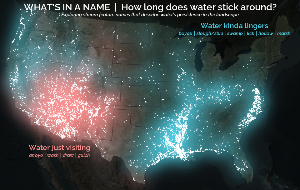
A map that glows with the vocabulary of water
What is your first impression of the map above? To me, it is the shimmer. Thousands of points of light, each one a stream or river, illuminating a darkened basemap. Look closely and a pattern emerges: the country’s waterways form a linguistic constellation. These points are classified not from population data or even explicitly by hydrology. They glow strictly according to the vocabulary used to name them and what can be implied about the hydrology of these streams based on their names.