
Large, parallel deep learning experiments using Snakemake
How we used Snakemake to automate and parallelize big deep learning experiments.
A paper we wrote was recently published! In the paper we had to run and evaluate many DL model runs. This post is all about how we automated these model runs and executed them in parallel using the workflow management software, Snakemake .
To multi-task or not to multi-task?
Before getting to Snakemake, we wanted to share some background about what exactly we were trying to do. In our paper, we asked (and started to answer) a somewhat basic question: is it helpful to multi-task? More specifically, we wondered if a deep learning model would be more accurate when trained to predict just one variable, streamflow, or when trained to predict two related variables, streamflow and water temperature? To answer this question, we designed a few experiments. Here we’ll focus on just one of four experiments - the one that required the most model runs. We used Snakemake for the other three experiments as well and found some interesting things from those too. If you are interested in the results of all four experiments, check out the full paper.
27,270 model runs
Our first experiment required 27,270 model runs! Let’s break that down.
- In the experiment we trained a separate DL model (LSTM) for each of 101 NWIS stations.
- For each station we needed to test the effect of a multi-task scaling factor to see how beneficial multi-tasking was; the larger the value of the multi-task scaling factor, the more the model focused on multi-tasking (predicting water temperature as well as streamflow) - the smaller the value, the more the model focused on just getting the primary task right (predicting streamflow). For the experiment we tried out 9 different values of the multi-task scaling factor.
- Because the starting weights of each model were random, not all of the differences between models could be attributed to differences in the multi-task scaling factor. To account for this, 30 models with different random starting weights were trained for each station/multi-task scaling factor combination.
When you sum that all up, that’s 101 sites x 9 multi-task scaling factors x 30 random starting weights = 27,270 total model runs.
All of these 27k+ model runs were independent of each other. For example, the model for site A with a multi-task scaling factor of 1 and the model for site B with multi-task scaling factor of 10 had no effect on each other. Because all of the model runs were independent, they could be trained in parallel.
Enter Snakemake
To keep track of the 27,270 model runs, not to mention the data preprocessing, the model prediction, and the model evaluation steps (an additional 40k+ independent tasks), and to execute those tasks in parallel, we used Snakemake.
Snakefile, rules, and the DAG: defining the workflow
Snakemake is a Make -like workflow management software tool. Snakemake (like Make) generates a user-specified target file or set of files from a user-defined workflow. A Snakemake workflow is written in a Snakefile, a plain-text file that uses a yaml -like structure. The Snakefile consists of a series of rules defining the steps to produce the final desired file(s) including steps to produce all of the intermediate files.
Each Snakemake rule defines:
- the
inputfiles - the
outputfiles - the processing step to produce the
outputfrom theinput
When you execute Snakemake, you ask it to produce one or more files.
Snakemake will look for a rule whose output file name matches the file(s) you asked it to create.
Once it finds the rule that creates the file you are asking for, Snakemake checks if the rule’s input files are created and up to date.
If the input files are not present or they are out of date, Snakemake will look for the rule(s) that produce those files and check their input files and so on.
In this way, Snakemake makes a directed acyclic graph (DAG)
that maps the entire process of getting the end products from the initial inputs, and through all intermediate steps.
Our workflow’s rules
Let’s look at an example from our Snakemake workflow.
Below is our evaluate_predictions rule.
It defines (1) model predictions and observation files as the input, (2) a metrics .csv file as the output, and (3) the calculate_metrics Python function in the run section as the processing step to use the input to produce the output.
rule evaluate_predictions:
    input:
        "expA/site_id_{site_id}/factor_{factor}/rand_seed_{seed}/{partition}_preds.csv",
        "obs_file.csv"
    output:
        "expA/site_id_{site_id}/factor_{factor}/rand_seed_{seed}/{partition}_metrics.csv"
    run:
        calculate_metrics(input[0], input[1], output[0], partition=wildcards.partition)
The curly braces are “wildcard” placeholders which we’ll talk more about later.
In addition to the evaluate_predictions rule, we defined
- the
prep_io_datarule to prepare our data for model training, - the
train_modelrule that used the prepared data (the output of theprep_io_datarule) to train the DL model, - and the
make_predictionsrule that took the trained model and the prepared data to make predictions.
Wildcards, expanding, and gathering: scaling to 27,270 branches
The prep_io_data rule was performed once for each of the 101 sites.
Then each site’s single prepared data file was used for each random initialization/multi-task scaling factor combination.
The train, predict, and evaluate rules, were applied to all 27,270 model runs.
These processes were the same for every observation site/multi-task scaling factor/random initialization combination.
Snakemake’s “wildcard” and “expand” functionalities allowed us to apply the same rules to all these combinations and keep track of them all.
We also defined a rule to gather all of the metric files for the final analysis.
Wildcards
Wildcards in Snakemake are placeholders in the output file definitions indicated by curly braces “{}”.
These wildcards tell Snakemake how to parse key information from filepaths given.
For example, the evaluate_predictions rule (above) had wildcards for site_id, factor (the multi-task scaling factor), seed, and partition.
With these wildcards, Snakemake can use the output file path to get the correct values to pass to the calculate_prediction function.
For example, if we asked Snakemake to produce "expA/site_id_01022500/factor_10/rand_seed_4/validation_metrics.csv", using the wildcards defined in the file structure, it would parse out the following:
site_id: “01022500”factor: “10”seed: “4”partition: “validation”
and it would make the following function call in the run step:
calculate_metrics("expA/site_id_01022500/factor_10/rand_seed_4/validation_preds.csv",
				  "obs_file.csv",
				  "expA/site_id_01022500/factor_10/rand_seed_4/validation_metrics.csv",
				  partition = "validation")
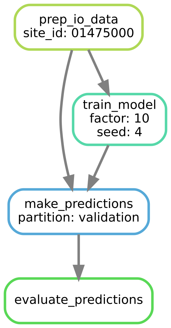
The DAG (directed acyclic graph) for producing performance metrics for one site, one multi-task scaling factor, and one random seed.
expanding
While wildcards are placeholders that make rules applicable to a single combination of inputs, the Snakemake expand function makes it easy to apply a rule (or set of rules) to all input combinations.
Instead of asking Snakemake to produce just one file (e.g., "expA/site_id_01022500/factor_10/validation_metrics.csv"), using expand, we succinctly ask Snakemake to produce all the files we need.
For example, to produce the validation prediction files for each site, multi-task scaling factor, and random seed, we would use expand like this:
expand("expA/site_id_{sites}/factor_{factors}/rand_seed_{seeds}/validation_metrics.csv"`,
		sites=all_sites,
		factors=all_factors,
		seeds=all_seeds)
where all_sites is the list of the 101 NWIS sites we were predicting at, all_factors the list of all of the multi-task scaling factors we were testing, and all_seeds the list of random seeds (0-29) that were used as random starting points.
The expand function makes filenames from all possible combinations of these three variables (i.e., 27,270) and Snakemake runs the workflow to produce each file.
Gathering
Once the 27,270 models were trained and the predictions were made and evaluated, we needed to “gather” all of the metrics into one file so we could compare performance across multi-task scaling factors.
For this gathering we wrote a combine_metrics rule.
rule combine_metrics:
    input:
		expand("expA/site_id_{sites}/factor_{factors}/rand_seed_{seeds}/validation_metrics.csv"`,
				sites=all_sites,
				factors=all_factors,
				seeds=all_seeds)
    output:
        "expA/overall_metrics.csv"
    run:
        combine_exp_metrics(input, output[0])
In this rule, the combine_exp_metrics Python function took the list of the 27,270 .csv files (produced by the expand function) and combined them into a new .csv file.
Finally, to let Snakemake know that the “overall_metrics.csv” file was the ultimate file we needed, we added this in the first rule of the Snakefile, all.
If no arguments are passed when calling Snakemake, it executes the first rule in the Snakefile. So in our case, it executed the all rule which means it looked for the “overall_metrics.csv” file. If “overall_metrics.csv” was not present and up to date, it then ran the necessary rules to produce that file.
rule all:
	input:
        "expA/overall_metrics.csv"
Below is the DAG for just two sites, two multi-task scaling factors, and two random seeds. This is representing just a small subset (8 model runs) of the full DAG. The full DAG, with all 27,270 model runs would be 3400 times wider!
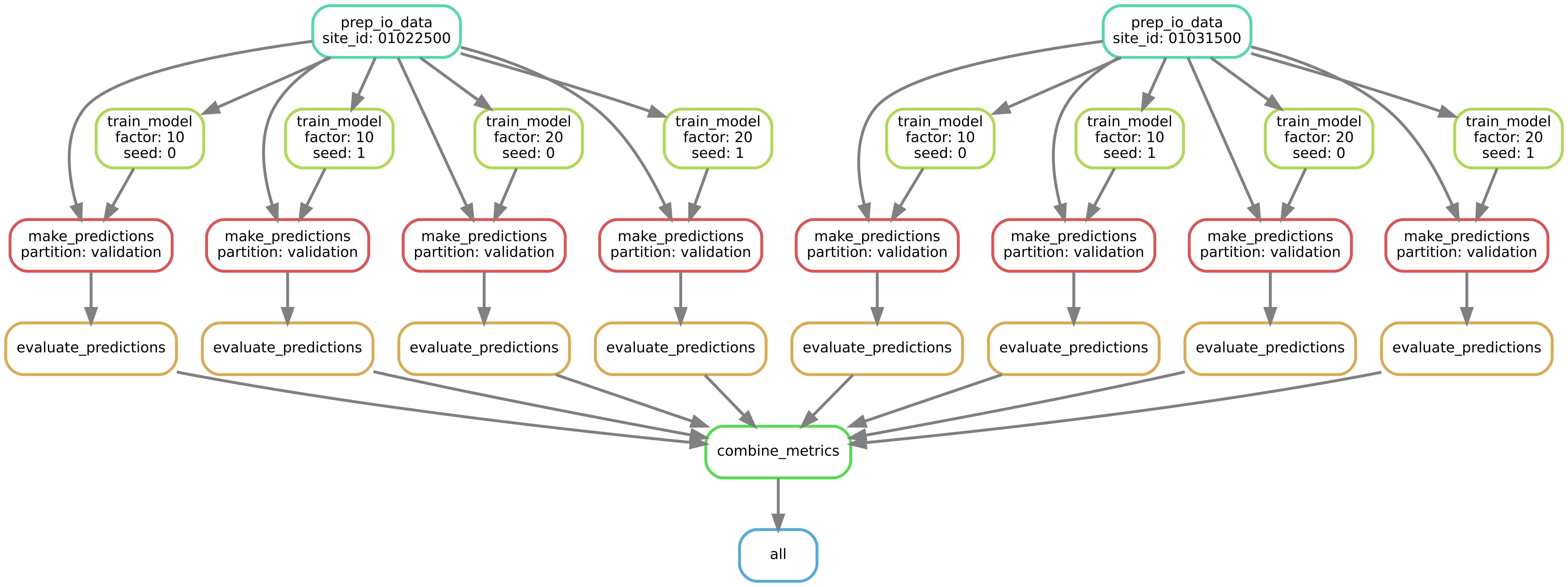
The DAG (directed acyclic graph) for producing performance metrics for two sites, two multi-task scaling factors, and two random seeds.
All of the tasks
When you run the workflow (-n in “dry” mode; and --quiet for a summary of the tasks)
snakemake -n --quiet
you get a summary of all the tasks (in alphabetical order):
Job counts:
        count   jobs
        1       all
        1       combine_metrics
        27270   evaluate_predictions
        27270   make_predictions
        101     prep_io_data
        27270   train_model
        81913
Executing Snakemake on many cores
To make this experiment, with its 80k tasks, doable in a reasonable time frame, we used Snakemake’s functionality for cluster execution. This allowed us to distribute these jobs for execution across many cores on the USGS high performance computer (HPC), Tallgrass. To run the workflow on the cluster, we did not have to change anything in our Snakefile. We only had to slightly modify the Snakemake execution command. The command on the HPC looked like this:
nohup snakemake --cluster "sbatch -A {cluster.account} -t {cluster.time} -p {cluster.partition} -N {cluster.nodes} -n 1 {cluster.gpu}" -p -k -j 400 --cluster-config ~/cluster_config.yml --rerun-incomplete --configfile config.yml -T 0 > run.out &
nohup let us start the job and then exit the terminal. The sbatch ... bit is the command that prefaced each job submission and the values for the {cluster.account} etc. were found in the cluster_config.yml* file. The -k flag is short for “keep going” meaning that if one job failed, independent jobs would still be submitted. And -j 400 meant that we were asking it to run 400 jobs at once (i.e., we were going to submit up to 400 jobs to the scheduler at a time). By running it on many cores at a time, it took only a couple of hours to churn through these 80k+ jobs and get our experiment results!
*the Snakemake documentation
says that the --cluster-config approach is deprecated in favor of using --profile.
When things didn’t work
As you may imagine, there were some hiccups in getting the workflow exactly right. Some of those hiccups were our errors. Some were other issues with the cluster. One critical advantage of using Snakemake, is that it checks to see if an output file is created and up to date before trying to create it. So, if 40% of the workflow ran before there was an error, the next time we ran Snakemake it would start running on just the parts that weren’t executed. This was an essential functionality with 80k+ jobs - otherwise, we’d only get the answer if it ran the whole workflow without a single error.
Wrapping up
Snakemake is a very powerful and flexible tool that allowed us to concisely define our large deep learning experiments. It also allowed us to easily execute that workflow (80k+ jobs) on a compute cluster. With Snakemake running on the USGS cluster our large experiments were executed in a less than a couple of hours. And anytime something went wrong with one of the 80k+ jobs, Snakemake knew to only re-run the affected jobs. With all of this functionality, Snakemake was a critical tool that let us get answers to our multi-task questions in a reasonable amount of time.
Endnotes
The workflows used for our paper
The workflows used for our paper are found in a ScienceBase data release that accompanies our manuscript. Note that for this blog post, we made some simplifications to the workflow to more clearly communicate the concepts.
The entire workflow
from utils import (prep_data, train, predict, calculate_metrics, combine_all_metrics, get_all_sites)

all_sites=get_all_sites()
all_factors = [0, 1, 5, 10, 20, 40, 80, 160, 320]
all_seeds = list(range(30))

rule all:
    input:
        "expA/overall_metrics.csv"


rule prep_io_data:
    input:
        "obs_file.csv",
        "input_file.csv"
    output:
        "expA/site_id_{site_id}/prepped_data.npz"
    run:
        prep_data(input, site=wildcards.site_id, out_file=output[0])


rule train_model:
    input:
        "expA/site_id_{site_id}/prepped_data.npz"
    output:
        "expA/site_id_{site_id}/factor_{factor}/rand_seed_{seed}/trained_model"
    run:
        train(input[0], factor=wildcards.factor, seed=wildcards.seed, out_file=output[0])


rule make_predictions:
    input:
        "expA/site_id_{site_id}/prepped_data.npz",
        "expA/site_id_{site_id}/factor_{factor}/rand_seed_{seed}/trained_model"
    output:
        "expA/site_id_{site_id}/factor_{factor}/rand_seed_{seed}/{partition}_preds.csv",
    run:
        predict(input[0], input[1], partition=wildcards.partition, out_file=output[0])


rule evaluate_predictions:
    input:
        "obs_file.csv",
        "expA/site_id_{site_id}/factor_{factor}/rand_seed_{seed}/{partition}_preds.csv",
    output:
        "expA/site_id_{site_id}/factor_{factor}/rand_seed_{seed}/{partition}_metrics.csv"
    run:
        calculate_metrics(input[0], input[1], partition=wildcards.partition, out_file=output[0])


rule combine_metrics:
    input:
        expand("expA/site_id_{sites}/factor_{factors}/rand_seed_{seeds}/validation_metrics.csv",
                sites=all_sites,
                factors=all_factors,
                seeds=all_seeds)
    output:
        "expA/overall_metrics.csv"
    run:
        combine_all_metrics(input, output[0])
Categories:
Related Posts
USGS water data science in 2022
September 3, 2022
The USGS water data science branch in 2022
The USGS data science branch advances environmental sciences and water information delivery with data-intensive modeling, data workflows, visualizations, and analytics. A short summary of our history can be found in a prior blog post . Sometimes I refer to data scientists as experts in wrangling complex data and making it more valuable or usable. I’m writing this blog to update readers on the types of things we’re up to and point out some future changes (including new hiring efforts).
TopoRivBlender - Create custom 3D images of Topography and Hydrography
September 18, 2025
Introduction
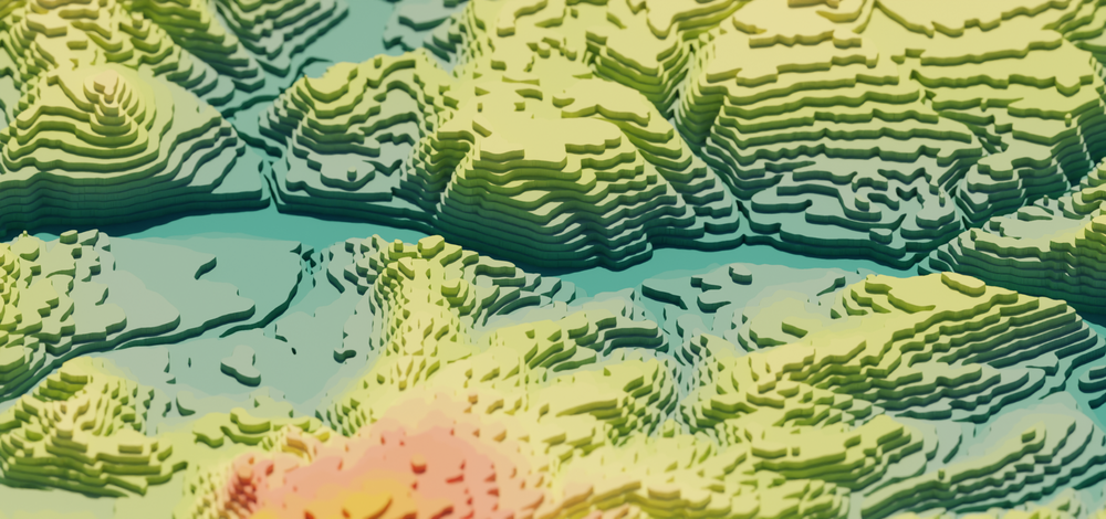
This blog will introduce you to an automated workflow that downloads geospatial data and then processes it to be used by 3D graphic software, Blender, to make images like the ones above and below. After reading through this blog, you should be able to use the example workflows to make your own images with just some basic coding knowledge. For Python users, this repository will also act as a starting point to make your own Blender workflows.
Participate in the EFI-USGS River Chlorophyll Forecasting Challenge!
April 22, 2024
We invite you to submit to the EFI-USGS River Chlorophyll Forecasting Challenge ! Co-hosted by the Ecological Forecasting Initiative (EFI) and U.S. Geological Survey (USGS) Proxies Project , this challenge provides a unique opportunity to forecast data from the USGS. By participating, you’ll sharpen your forecasting skills and contribute to vital research aimed at addressing pressing environmental concerns, such as harmful algal blooms (HABs) and water quality.
Water Data Science in 2021
March 5, 2021
Where the USGS Water Data Science Branch is headed in 2021
It is an exciting time to be a data science practitioner in environmental science. In the last five years, we’ve seen massive data growth, modeling improvements, new more inclusive definitions of “impact” in science, and new jobs and duties. The title of “data scientist” has even been formally added as a job role by the federal government and there are all kinds of data science needs spelled out in the new USGS science plan .