
TopoRivBlender - Create custom 3D images of Topography and Hydrography
Reproducible workflows that provide the data and tools for you to get started making your own 3D graphics of topographic, satellite, and water data
What's on this page
Introduction
This blog will introduce you to an automated workflow that downloads geospatial data and then processes it to be used by 3D graphic software, Blender, to make images like the ones above and below. After reading through this blog, you should be able to use the example workflows to make your own images with just some basic coding knowledge. For Python users, this repository will also act as a starting point to make your own Blender workflows.
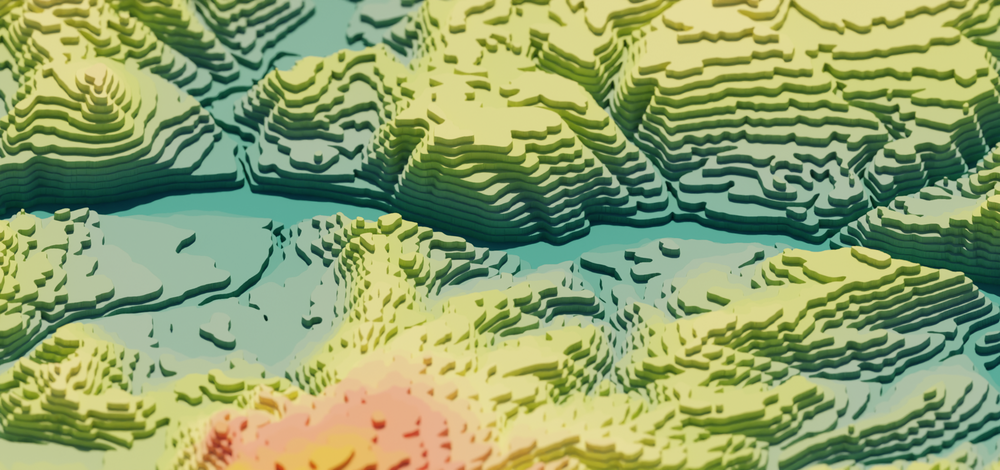
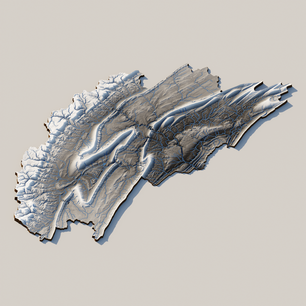
A rendered 3D image of topography, hydrography, and satellite imagery around Kings Peak in Utah, USA.
topo-riv-blender
topo-riv-blender contains Python functions and workflows that allow for reproducible, automated generation of 3-dimensional images.
The workflow is coded using a snakemake
workflow that will programmatically (a) download geospatial data, (b) create 3-dimensional (3D) objects in Blender, and (c) generate the rendered image, all in just a few minutes.
Rendering is the process of using your computer’s CPU (central processing unit) or GPU (graphics processing unit) to predict how light bounces off 3D objects into a simulated camera to make an image; think of it like setting a scene (an object and light source) and taking a picture.
topo
The topo part of this workflow’s name stands for topography.
Topographic data tells us the height (or elevation) of the Earth’s surface.
When this data is recorded in a digital form, it is often referred to as a Digital Elevation Model (DEM).
DEMs are commonly saved as raster files, which is a gridded dataset.
Like a digital photograph that is made of many colored pixels, each pixel in a DEM contains the height or elevation of the Earth’s surface.
More about USGS topography data
3DEP
The USGS manages the 3D Elevation Program (3DEP), which aims to build "high-quality topographic data and three-dimensional (3D) representations of the Nation's natural and constructed features." At the time of writing the blog (Sept 2025), 3DEP coverage over the entire U.S. is nearly complete. In many locations, multiple DEMs made at different times have been created, allowing scientists to study how the Earth's surface changes over time.
riv
The riv part of this workflow’s name stands for river network.
River network data tells us where streams and rivers flow and connect.
The locations of river and surface water are commonly saved as vector files.
In these vector files, river pathways are represented as a series of lines that connect to one other on the Earth’s surface.
More about USGS hydrography data
NHD and 3DHP
The study of the location of river networks as well as other water features (e.g., lakes, ponds, oceans) is called hydrography. The USGS developed the National Hydrography Dataset (NHD), representing the planform (2D) geometry of the United States' water resources. Since October 1st, 2023, NHD is still available but is no longer maintained. The next generation of hydrography data will be contained in the 3D Hydrography Program (3DHP).
blender
Blender
is a free and open-source 3D graphics software that you can use to create photorealistic images.
In this workflow, we use Python to process the geospatial data for Blender to create the 3D images.
We also utilize the Blender Python API to render images with code.
Setting up topo-riv-blender
You will need to set up a few things on your computer before getting started.
topo-riv-blender will work on multiple operating systems.
Essentially, you will need two programs, Miniforge (or another conda package manager, e.g. Anaconda) and Blender.
If you already have these programs, you can skip some of the steps, but you might want to make sure they are up to date.
- macOS and Linux users, please start with Step A1
- Windows users, please start with Step A2.
Step A1: macOS and Linux installation
- Download and install Blender.
- Install Homebrew
, a package manager for macOS and Linux.
/bin/bash -c "$(curl -fsSL https://raw.githubusercontent.com/Homebrew/install/HEAD/install.sh)" - Install Miniforge.
brew install --cask miniforge - Go to Step B.
Step A2: Windows installation
- Download and install Git Bash.
- Download and install Miniforge.
- Initialize
conda,- From the Start menu, open
Miniforge Prompt
- Type and execute
conda init bash
- This allows you to use
condain Git Bash.
- From the Start menu, open
- Install Blender.
- NOTE: Be sure to remember where Blender is installed.
- At the time of writing this blog,
4.4is the latest version, which typically installs inC:\Program Files\Blender Foundation\Blender 4.4
- Add Blender to
PATHby editing the~/.bash_profile- Open Git Bash by right-clicking on the Desktop and selecting Git Bash Here
- Edit the
~/.bash_profilefile by typing and executingnano ~/.bash_profile
- Paste the following line inside
~/.bash_profileexport PATH=$PATH:"/c/Program Files/Blender Foundation/Blender 4.4".- NOTE: Adjust the directory based on where Blender is installed on your machine. Also, make sure to adjust the version number accordingly.
- Go to Step B.
Step B: Check your installation
- Before moving on, check that you can access
condain terminal (macOS/Linux) or Git Bash (Windows)- Type and execute
conda- After executing, options for using this command should show appear.
- Type and execute
- You should check that you can access Blender in terminal (macOS/Linux) or Git Bash (Windows)
- Type and execute
Blender- After executing, the Blender program should open.
- Typically, we will use Blender in the background (i.e., without the UI).
- Type and execute
Step C: Download topo-riv-blender
- If you have a GitHub account, you can git clone or fork the
topo-riv-blenderrepository, found here: https://github.com/DOI-USGS/topo-riv-blender . - If you do not have a GitHub account, you can download the entire repository from this link .
- Unzip the file and move the directory to your desired location. Make note of the path, e.g.,
cd path/to/topo-riv-blenderorcd path/to/topo-riv-blender-main. - This directory will be the project folder where you download, process, and visualize the data in the pipeline.
Step D: Set up the conda environment
- In the terminal (macOS/Linux) or Git Bash (Windows) change directories to the project directory with
cd path/to/topo-riv-blender. - Create the
condaenvironment using theenvironment.yamlfile. Runconda env create -f environment.yaml. - Activate the conda environment.
Run
conda activate topo-riv-blender.
Step E: Get an API key from OpenTopography
- Request an API key from OpenTopography.
- It’s free and will allow you to access many different topographic datasets .
- Make an account here .
- Click the “Request API Key” button on this page when logged in.
- When you get the key, return to this page and you will see a text string that you can copy for Step 2.
- Create a
.txtfile namedopentopography_api_key.txtinpath/to/topo-riv-blenderand paste your API key in it.
Making your first 3D image
Now that everything is set up on your computer, let’s create some 3D images.
Here, we use snakemake,
a workflow management system that helps organize the data and processes required to make the 3D images.
A workflow used to process and organize data is commonly referred to as a data pipeline or just pipeline.
In the command-line (terminal for macOS and Linux users, Git Bash for Windows users), type the following command:
snakemake --cores 1 -s Snakefile phase_2_visualize/out/render_02050302.png
This should make the following image, located in:
phase_2_visualize/out/render_02050302.png
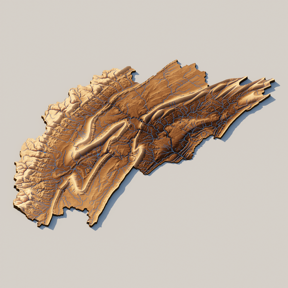
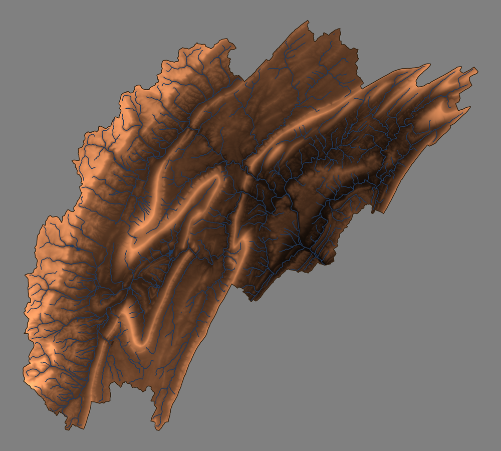
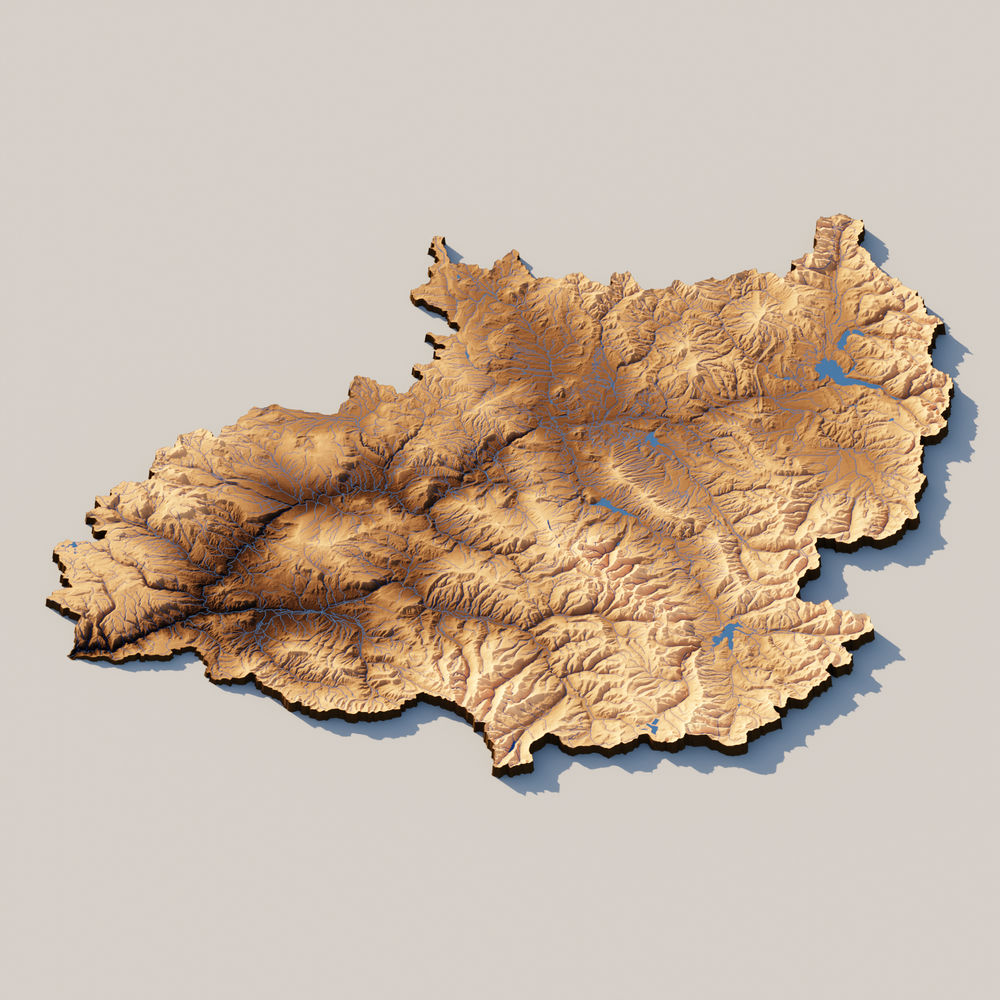
A rendered 3D image of topography and hydrography in Upper Juniata in Central Pennsylvania (HUC: 02050302).
Let’s break down the command:
snakemake: used to call thesnakemakeworkflow manager--cores 1: determines the number of cores to use on your computer to speed up the pipeline. You can use more than one to run the workflow in parallel or useallto use all available cores.-s Snakefile: determines whichSnakefileto use. In the main directory, you will see otherSnakefiles, which contain workflows to make other 3D visualizations, e.g.,Snakefile_countour. Note: If you do not write this argument,snakemakewill default to the file namedSnakefile.phase_2_visualize/out/render_02050302.png: determines the file path for the final 3D image file. You can change this to create different 3D visualizations. The 8-digit number,02050302, is a Hydrologic Unit Code (HUC), which identifies a landscape area that drains water.
What does the Snakefile pipeline do?
When you call the command, the snakemake pipeline works backward, gathering and processing everything it needs to create the 3D visualization.
Below, we will go over the three major phases/steps of the pipeline in Snakefile, which is located in the main directory.
This is just a brief overview of the processes and parameters within the pipeline.
For more information, please visit the README.md
in the topo-riv-blender GitHub repo.
Phase 1: Fetch
To create the visual (render_02050302.png), we first need to gather the necessary geospatial data.
Based on the user’s specified output, the pipeline uses the HUC8 value, 02050302, to download the following:
- a polygon of the HUC8,
02050302(.shp) - a topographic raster (a black-and-white image) within the HUC8 polygon (.tif)
- a collection of river and stream lines within the HUC8 polygon (.shp)
- a collection of waterbody polygons (e.g. lakes, ponds, reservoirs) within the HUC8 polygon (.shp)
Phase 2: Process
The data needs to be translated in order for Blender to make a 3D visualization. Blender only requires two inputs, a height map and a texture map.
The height map is a black and white image that shows the elevation at all locations in the landscape. Darker regions are lower elevation, and lighter regions are higher elevations. This image is essentially the same as the topographic raster or DEM. This image will help Blender create the shape of the topography.
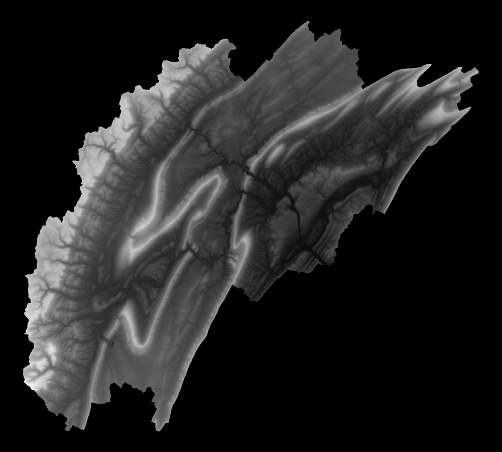
Height map of the landscape.
The texture map is a color image that determines the color of the landscape’s surface. For this image, we specify a color map to represent the elevation. The default parameters use light and dark brown regions to highlight higher and lower elevations, respectively. We also use this image to map out river lines and waterbody polygons. This image will help Blender create the color of the topography.
Texture map of the landscape.
Phase 3: Visualize
We then import the height map and texture map into Blender. It will create a plane and then modify the shape of its surface to match the topography in the height map. We also add a fake “sun” to light the geometry and create the appealing shadows.
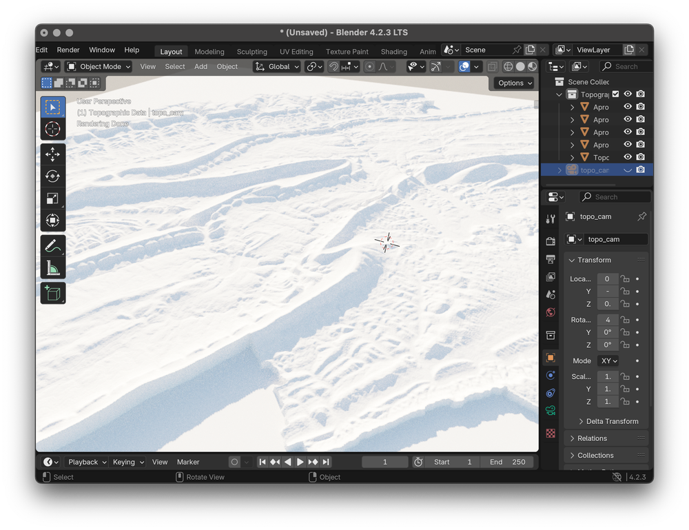
Height map of the landscape displayed in the Blender UI.
Next, we overlay the texture map on top of the topography, coloring the geometry. The light and dark browns help highlight the shape of the landscape and the blue lines denote the river pathways.
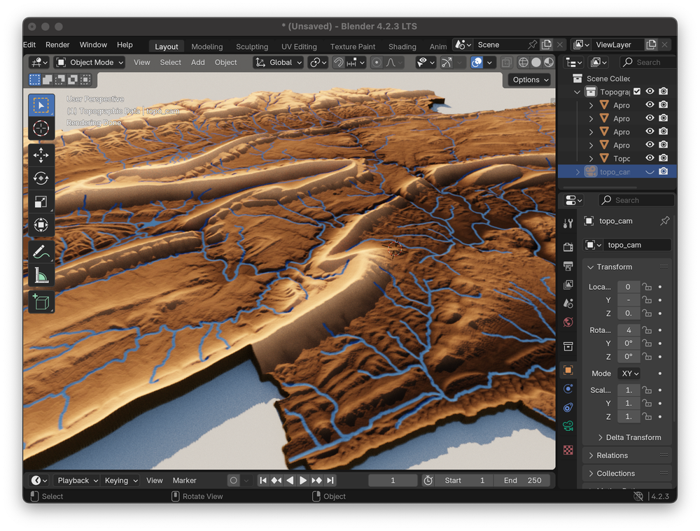
Texture map overlaying the height map in the Blender UI.
How to use the default Snakefile
snakemake allows you to create a flexible data pipeline that can fetch, process, and visualize many different locations.
Method 1: Command-line interface
The default Snakefile is meant to create 3D visualizations of topography and hydrography at any HUC of your choosing.
Here are some example commands that you can use.
Specifying a different HUC
Do you want to make a render of a HUC12, 070400030309?
You can specify this new output to generate the render.
snakemake --cores 1 -s Snakefile phase_2_visualize/out/render_070400030309.png
Render of HUC - 070400030309
Specifying multiple HUCs, separately
You can use the workflow to create multiple 3D images by specifying all output images in a single command.
Make sure to add a space between the image paths.
Below, we create separate images for three HUC8s: 14010001, 14010002, and 14010003.
snakemake --cores 1 -s Snakefile phase_2_visualize/out/render_14010001.png phase_2_visualize/out/render_14010002.png phase_2_visualize/out/render_14010003.png
Render of HUC - 14010001
Render of HUC - 14010002
Render of HUC - 14010003
Specifying multiple HUCs together
You can combine the HUCs within the same 3D visualization.
Type the word and in between each HUC.
Below, we create a single image of the three HUC8s: 14010001, 14010002, and 14010003.
snakemake --cores 1 -s Snakefile phase_2_visualize/out/render_14010001and14010002and14010003.png
Render of HUCs - 14010001, 14010002, and 14010003, combined
Method 2: Modifying the Snakefile set the outputs
Let’s take a peek inside the Snakefile.
You will see a section called rule all.
The Snakefile included in topo-riv-blender contains three different HUCs, 140100, 02050302, and 070400030309 in rule all.
See the code: Snakefile
# Render Parameters File
module_name = "blender_parameters.blender_params_auto"

# Import parameters file
import os, sys, importlib
render_params = module_name.replace(".", os.sep) + ".py"
parameters = importlib.import_module(module_name)

# Define the final outputs
rule all:
    input:
        "phase_2_visualize/out/render_140100.png",
        "phase_2_visualize/out/render_02050302.png",
        "phase_2_visualize/out/render_070400030309.png"

###################################################################################
# PHASE 1: FETCH ##################################################################
###################################################################################

# Downloads a shapefile of the HUC boundary
rule get_wbd:
    params:
        huc_list = lambda wildcards: f"{wildcards.huc_id}".split("and")
    output:
        extent_shpfile = "phase_0_fetch/out/{huc_id}/extent.shp"
    script:
        "phase_0_fetch/src/get_wbd.py"

# Downloads NHD flowline data within extent
rule get_nhd_fl:
    params:
        nhd_type = parameters.nhd_flowline,
        render_pixels = parameters.res_x * parameters.res_y
    input:
        extent_shpfile = "phase_0_fetch/out/{huc_id}/extent.shp"
    output:
        nhd_shpfile = "phase_0_fetch/out/{huc_id}/rivers.shp"
    script:
        "phase_0_fetch/src/get_nhd.py"

# Downloads NHD waterbody data within extent
rule get_nhd_wb:
    params:
        nhd_type = parameters.nhd_waterbody,
        render_pixels = parameters.res_x * parameters.res_y
    input:
        extent_shpfile = "phase_0_fetch/out/{huc_id}/extent.shp"
    output:
        nhd_shpfile = "phase_0_fetch/out/{huc_id}/waterbody.shp"
    script:
        "phase_0_fetch/src/get_nhd.py"

# Downloads a digital elevation model within extent
rule download_dem:
    params:
        dem_product = parameters.dem_product,
        buffer = parameters.buffer,
        render_pixels = parameters.res_x * parameters.res_y
    input:
        extent_shpfile = "phase_0_fetch/out/{huc_id}/extent.shp"
    output:
        demfile = "phase_0_fetch/out/{huc_id}/dem.tif"
    script:
        "phase_0_fetch/src/download_dem.py"

###################################################################################
# PHASE 2: PROCESS ################################################################
###################################################################################

# Creates a grayscale height map and texture map for Blender to render.
# The height map is used to determine how high the landscape should be
# in the render, and the texture map determines the color of the landscape.
rule create_heightmap_texturemap:
    params:
        buffer = parameters.buffer,
        topo_cmap = parameters.topo_cmap,
        background_color = parameters.background_color,
        wall_color = parameters.wall_color,
        river_color = parameters.river_color
    input:
        extent_shpfile = "phase_0_fetch/out/{huc_id}/extent.shp",
        demfile =  "phase_0_fetch/out/{huc_id}/dem.tif",
        flowlines_shpfile = "phase_0_fetch/out/{huc_id}/rivers.shp",
        waterbody_shpfile = "phase_0_fetch/out/{huc_id}/waterbody.shp"
    output:
        dimensions_file = "phase_1_process/out/{huc_id}/dimensions.npy",
        heightmap_file = "phase_1_process/out/{huc_id}/heightmap.png",
        texturemap_file = "phase_1_process/out/{huc_id}/texturemap.png",
        apronmap_file = "phase_1_process/out/{huc_id}/apronmap.png"
    script:
        "phase_1_process/src/process.py"

###################################################################################
# PHASE 3: VISUALIZE ##############################################################
###################################################################################

# Using the height map and texture map, Blender sets up the scene
# (topography, lighting, and camera) and renders a photorealistic image.
rule render:
    input:
        dimensions_file = "phase_1_process/out/{huc_id}/dimensions.npy",
        heightmap_file = "phase_1_process/out/{huc_id}/heightmap.png",
        texturemap_file = "phase_1_process/out/{huc_id}/texturemap.png",
        apronmap_file = "phase_1_process/out/{huc_id}/apronmap.png",
        blender_params = render_params
    output:
        output_file = "phase_2_visualize/out/render_{huc_id}.png"
    shell:
        "Blender -b -P phase_2_visualize/src/render.py -- "
        "{input.blender_params} "
        "{input.dimensions_file} {input.heightmap_file} {input.texturemap_file} {input.apronmap_file} NULL "
        "{output.output_file} "
If you run the following command:
snakemake --cores 1 -s Snakefile
snakemake, by default, will make those three images of the HUCs.
You can modify the Snakefile to include or exclude other HUC image paths instead of specifying the image paths in the command-line.
Hint: Want to use a bounding box to define your map region? Take a look at the examples below, and learn how to modify the bounding box to a location of your choosing.
Customizing the look of the 3D visualizations
Do you want to change the look of the visuals?
With this workflow, you can easily change the color of the topography, rivers, or background.
You can also adjust the lighting, camera settings, angle, etc.
The blender_parameters directory houses parameter files that you can modify to change the look of the rendered image.
Let’s take a look at the file named blender_params_auto.py in this directory.
See the parameters: blender_parameters/blender_params_auto.py
# For more details about the parameters, please refer to the README in the Github repository:
# https://github.com/DOI-USGS/topo-riv-blender/blob/main/README.md

########## data management ##########
# OpenTopography Products: https://portal.opentopography.org/apidocs/
dem_product = "auto"  # determine automatically (see options here: https://portal.opentopography.org/apidocs/#/)

# NHD products
nhd_flowline = "flowline_auto"  # use auto, mr, or hr
nhd_waterbody = "waterbody_auto"  # use auto, mr, or hr

# Data Buffer
buffer = 1.0  # percent buffer space around watershed

########## map visualization ##########
background_color = [0.5, 0.5, 0.5, 1.0]  # rgba color of the background
wall_color = [0.2, 0.133, 0.0667, 1.0]  # rgba color of the wall edge
river_color = [0.1294, 0.2275, 0.3608, 1.0]  # rgba color of the rivers
topo_cmap = "copper"  # color map of the topography, choose others here: https://matplotlib.org/stable/users/explain/colors/colormaps.html

########## render hardware ##########
GPU_boolean = False  # if you have a GPU, set this to 1 and this will run faster

########## blender scene ##########
# max dimension of plane
plane_size = 1.0  # meters, size of topography. Tt can be anything, but you need to position your camera accordingly.

########## additional data layers ##########
number_of_layers = 0  # number of additional data layers

########## camera settings ##########
# color management
view_transform = "Filmic"  # 'Standard'
exposure = 0.0  # default is 0, -2.0 to 2.0 will make image lighter to darker
gamma = 0.65  # default is 1, 0.25 to 2.0 will make the shadow areas lighter to darker

# camera type
camera_type = "orthogonal"  # orthogonal or perspective

# orthogonal
ortho_scale = 1.0  # when using orthogonal scale, increase to "zoom" out

# perspective
focal_length = 50.0  # mm when using perspective camera, increase to zoom in

# camera location
camera_distance = 1.0  # meters from the center (maximum horizontal axis is assumed to be 1 meter), this needs to be a similar value to the plane_size.
camera_tilt = (
    45.0  # degrees from horizontal: 0.0 is profile view, 90.0 is planform view
)
camera_rotation = 180.0  # camera location degrees clockwise from North: 0.0 is North, 90.0 is East, 180.0, is South, and 270.0 is West.
shift_x = 0.0  # you may need to shift the camera to center the topo in the frame, use small increments like 0.01
shift_y = 0.0  # you may need to shift the camera to center the topo in the frame, use small increments like 0.01

# depth of field
use_depth_of_field = (
    False  # makes things fuzzy when objects are away from the focal plane
)
dof_distance = camera_distance  # where the focal plane is
f_stop = 100.0  # affects depths of field, lower for a shallow dof, higher for wide dof

########## sun properties ##########
sun_tilt = 20.0  # degrees from horizontal
sun_rotation = 315.0  # degrees clockwise from North
sun_intensity = 0.5  # sun intensity, use small increments like 0.1 to adjust
sun_strength = 1.0  # sun strength, use small increments like 0.1 to adjust

########## landscape representation ###########
min_res = 2000  # minimum resolution of the heightmap, larger value increases detail but takes longer to render
number_of_subdivisions = 2000  # number of subdivisions, larger value increases detail but takes longer to render
exaggeration = "auto"  # vertical exaggeration
displacement_method = "DISPLACEMENT"  # "BOTH" #for more exaggerated shadows

########## render settings ##########
res_x = 2000  # x resolution of the render, larger value increases detail but takes longer to render
res_y = 2000  # y resolution of the render, larger value increases detail but takes longer to render
samples = 10  # number of samples that decides how "good" the render looks, larger value increases detail but takes longer to render
For a more detailed look at every parameter that can be changed, please take a look at the README.md file. Now, let’s walk through a few examples.
Change the color map of the topography
The default color map is matplotlib’s copper color map.
You can easily specify a different named matplotlib color map, which can be found here.
Let’s try a grayscale color map.
In the blender_parameters/blender_params_auto.py, change topo-cmap to:
topo_cmap = "grey"
A rendered 3D image of topography and hydrography in Upper Juniata in Central Pennsylvania (HUC: 02050302) with a grayscale color map.
Change the camera parameters
Let’s change the camera from an orthogonal
to a perspective viewpoint.
We can change the focal_length from 50mm to 250mm, giving the camera one of those large lenses that photographers use.
If we change the camera_tilt from 45 to 30, we can angle the camera slightly less downward.
Adjusting shift_y moves the camera upward (positive value) or downward (negative value).
Last, we use depth_of_field == True and f_stop = 5.0 to allow parts of the image outside the focal length to be out of focus (blurry).
Why make things out of focus?
It can help emphasize parts of the image and give the image an interesting aesthetic.
camera_type = "perspective"

focal_length = 250.0

camera_tilt = 30.0

shift_y = 0.25

use_depth_of_field = True

f_stop = 5.0
A rendered 3D image of topography and hydrography in Upper Juniata in Central Pennsylvania (HUC: 02050302) using a perspective viewpoint.
topo-riv-blender Gallery: Example workflows!
In topo-riv-blender, I have also included other Snakefiles with different functionalities.
See the gallery below!
Adding satellite imagery
Using the snakemake organization, I created fetching functions that can help you download global satellite imagery, such as Landsat, Sentinel, and MODIS.
Instead of specifying a HUC extent, this workflow requires the user to specify a bounding box (the coordinates of the upper-left and lower-right corners of the box).
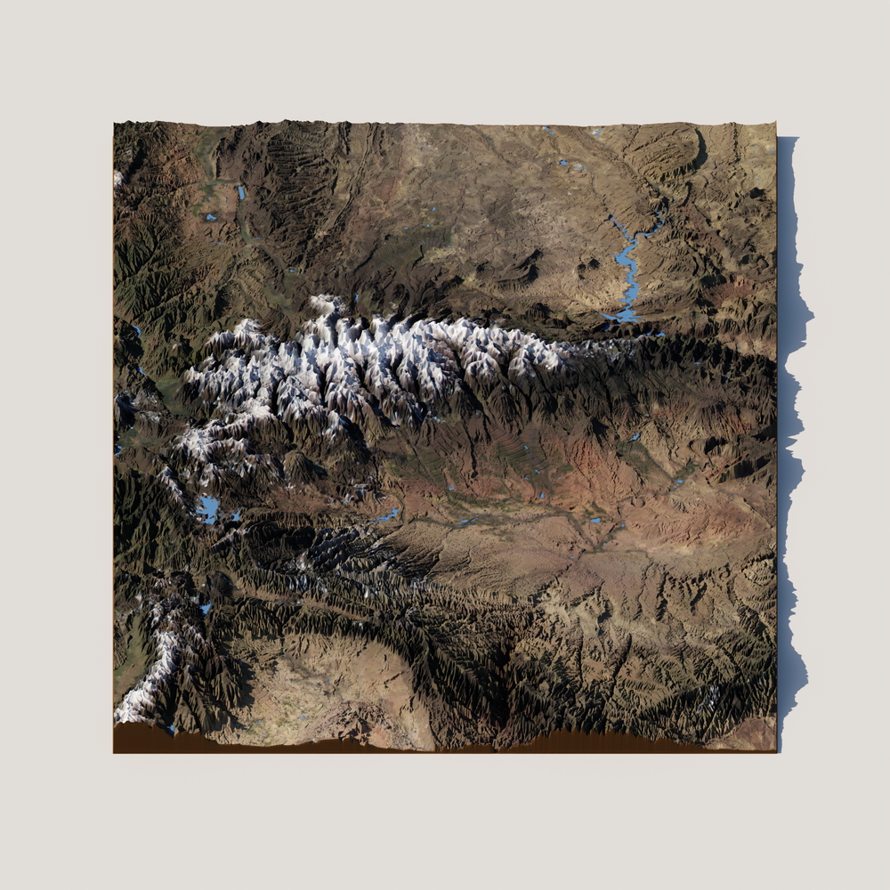
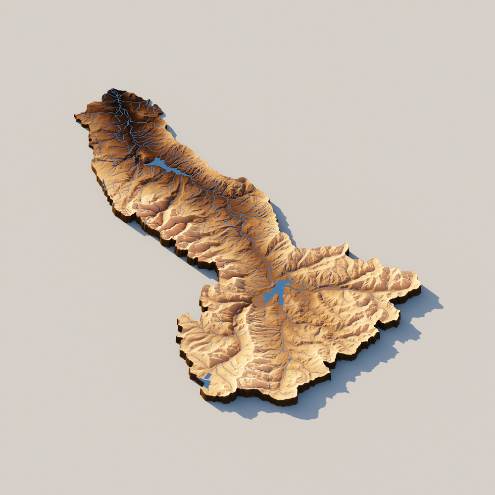
3D visualization of Kings Peak in Northeast Utah, USA.
snakemake --cores 1 -s Snakefile_aerial
See the code: Snakefile_aerial
Adding satellite imagery requires a bit of iteration.
Some images during certain periods may have too many clouds or artifacts.
You can adjust the temporal search window by changing the following start_query and end_query:
start_query="2024-05-01T14:00:00Z",
end_query="2024-05-30T20:00:00Z",
This query searches from May 1st, 2024 to May 30th, 2024 between times of 8:00am to 2:00pm local time.
If you want to use a different satellite than MODIS, consider changing the collection_id, see available collections here
.
target_asset_keys will also need to be adjusted to reflect the collection band names.
For simplicity and larger areas, I would stick with MODIS.
# Render Parameters File
module_name = "blender_parameters.blender_params_aerial"

# Import parameters file
import os, sys, importlib
render_params = module_name.replace(".", os.sep) + ".py"
parameters = importlib.import_module(module_name)

# Define the final output
rule all:
    input:
        "phase_2_visualize/out/render_kingspeak.png"

# Make the bounding box
rule make_bounding_box:
    params:
        UL_corner = [41.75, -111.5],
        LR_corner = [39.25, -109.0],
    output:
        extent_shpfile = "phase_0_fetch/out/{name}/extent.shp"
    script:
        "phase_0_fetch/src/make_bounding_box.py"

# Downloads a digital elevation model within extent
rule download_dem:
    params:
        dem_product = parameters.dem_product,
        render_pixels = parameters.res_x * parameters.res_y,
        buffer = parameters.buffer
    input:
        extent_shpfile = "phase_0_fetch/out/{name}/extent.shp"
    output:
        demfile = "phase_0_fetch/out/{name}/dem.tif"
    script:
        "phase_0_fetch/src/download_dem.py"

# Downloads aerial imagery within extent
target_asset_keys = ["sur_refl_b01", "sur_refl_b04", "sur_refl_b03"]
rule download_aerial:
    params:
        collection_id = "modis-09A1-061",
        target_asset_keys = target_asset_keys,
        start_query="2024-05-01T14:00:00Z",
        end_query="2024-05-30T20:00:00Z",
    input:
        extent_shpfile =  "phase_0_fetch/out/{name}/extent.shp"
    output:
        out_bands = ["phase_0_fetch/out/{name}/" + band + ".tif" for band in target_asset_keys]
    script:
        "phase_0_fetch/src/get_imagery.py"

# sharpen
rule sharpen:
    params:
        upsample = 2,
        method = 'cubic'
    input:
        input_bands = ["phase_0_fetch/out/{name}/" + band + ".tif" for band in target_asset_keys]
    output:
        output_bands = ["phase_0_fetch/out/{name}/" + band + "_sharp.tif" for band in target_asset_keys]
    script:
        "phase_1_process/src/upsample.py"

# Downloads NHD flowline data within extent
rule get_nhd_fl:
    params:
        nhd_type = parameters.nhd_flowline,
        render_pixels = parameters.res_x * parameters.res_y
    input:
        extent_shpfile = "phase_0_fetch/out/{name}/extent.shp"
    output:
        nhd_shpfile = "phase_0_fetch/out/{name}/rivers.shp"
    script:
        "phase_0_fetch/src/get_nhd.py"

# Downloads NHD waterbody data within extent
rule get_nhd_wb:
    params:
        nhd_type = parameters.nhd_waterbody,
        render_pixels = parameters.res_x * parameters.res_y
    input:
        extent_shpfile =  "phase_0_fetch/out/{name}/extent.shp"
    output:
        nhd_shpfile = "phase_0_fetch/out/{name}/waterbody.shp"
    script:
        "phase_0_fetch/src/get_nhd.py"

# filter out small streams in nhd data
rule filter_streams:
    params:
        min_stream_order = 4 #lambda wildcards: min_stream_orders[wildcards.name]
    input:
        nhd_shpfile = "phase_0_fetch/out/{name}/rivers.shp"
    output:
        filtered_nhd_shpfile = "phase_0_fetch/out/{name}/filtered_rivers.shp"
    script:
        "phase_1_process/src/filter_streams.py"

# Creates a grayscale height map and texture map for Blender to render.
# The height map is used to determine how high the landscape should be
# in the render, and the texture map determines the color of the landscape.
rule create_heightmap_texturemap:
    params:
        map_crs = "EPSG:3857",
        buffer = parameters.buffer,
        wall_thickness = 1.5,
        wall_color = [0.2, 0.133, 0.067, 1.0],
        background_color = [0.5, 0.5, 0.5, 1.0]
    input:
        extent_shpfile =  "phase_0_fetch/out/{name}/extent.shp",
        demfile =  "phase_0_fetch/out/{name}/dem.tif",
        aerialfiles =  ["phase_0_fetch/out/{name}/" + band + "_sharp.tif" for band in target_asset_keys],
        flowlines_shpfile = "phase_0_fetch/out/{name}/filtered_rivers.shp",
        waterbody_shpfile = "phase_0_fetch/out/{name}/waterbody.shp"
    output:
        dimensions_file = "phase_1_process/out/{name}/dimensions.npy",
        heightmap_file = "phase_1_process/out/{name}/heightmap.png",
        texturemap_file = "phase_1_process/out/{name}/texturemap.png",
        apronmap_file = "phase_1_process/out/{name}/apronmap.png"
    script:
        "phase_1_process/src/process.py"

# Using the height map and texture map, Blender sets up the scene
# (topography, lighting, and camera) and renders a photorealistic image.
rule render:
    input:
        dimensions_file = "phase_1_process/out/{name}/dimensions.npy",
        heightmap_file = "phase_1_process/out/{name}/heightmap.png",
        texturemap_file = "phase_1_process/out/{name}/texturemap.png",
        apronmap_file = "phase_1_process/out/{name}/apronmap.png",
        blender_params = render_params
    output:
        output_file = "phase_2_visualize/out/render_{name}.png"
    shell:
        "Blender -b -P phase_2_visualize/src/render.py -- "
        "{input.blender_params} "
        "{input.dimensions_file} {input.heightmap_file} {input.texturemap_file} {input.apronmap_file} NULL "
        "{output.output_file} "
See the parameters: blender_parameters/blender_params_aerial.py
# For more details about the parameters, please refer to the README in the Github repository:
# https://github.com/DOI-USGS/topo-riv-blender/blob/main/README.md

########## data management ##########
# OpenTopography Products: https://portal.opentopography.org/apidocs/
data_product = "/API/usgsdem"  # <- USGS datasets
dem_product = "auto"  # auto
buffer = 0.2  # buffer space around watershed
# NHD products
nhd_flowline = "flowline_mr"  # use auto, mr, or hr
nhd_waterbody = "waterbody_mr"  # use auto, mr, or hr

########## map visualization ##########

# topography colormap
topo_cmap = "copper"

########## render hardware ##########
GPU_boolean = False  # if you have a GPU, set this to 1 and this will run faster

########## blender scene ##########
# max dimension of plane
plane_size = 1.0  # meters

########## additional data layers ##########
number_of_layers = 0  # number of additional data layers

########## camera settings ##########
# color management
view_transform = "Filmic"  # 'Standard'
exposure = -0.75  #'default is 0
gamma = 0.75  # default is 1

# camera type
camera_type = "orthogonal"  # orthogonal or perspective

# orthogonal
ortho_scale = 1.0  # when using orthogonal scale, increase to "zoom" out

# perspective
focal_length = 50.0  # mm when using perspective camera, increase to zoom in
shift_x = 0.0  # you may need to shift the camera to center the topo in the frame
shift_y = 0.0  # you may need to shift the camera to center the topo in the frame

# camera location
camera_distance = (
    1.0  # meters from the center (maximum horizontal axis is assumed to be 1 meter)
)
camera_tilt = (
    45.0  # degrees from horizontal: 0.0 is profile view, 90.0 is planform view
)
camera_rotation = 180.0  # camera location degrees clockwise from North: 0.0 is North, 90.0 is East, 180.0, is South, and 270.0 is West.

# depth of field
use_depth_of_field = False
dof_distance = camera_distance  # where the focal plane is
f_stop = 100.0  # affects depths of field, lower for a shallow dof, higher for wide dof

########## sun properties ##########
sun_tilt = 45.0  # degrees from horizontal
sun_rotation = 270.0  # degrees clockwise from North
sun_intensity = 0.5  # sun intensity
sun_strength = 1.0  # sun strength

########## landscape representation ###########
min_res = 2000  # minimum resolution of the height map, larger value increases detail but takes longer to render
number_of_subdivisions = 2000  # number of subdivisions, larger value increases detail but takes longer to render
exaggeration = 10.0  # vertical exaggeration
displacement_method = "DISPLACEMENT"  # "BOTH" #for more exaggerated shadows

########## render settings ##########
res_x = 2500  # x resolution of the render, larger value increases detail but takes longer to render
res_y = 2500  # y resolution of the render, larger value increases detail but takes longer to render
samples = 10  # number of samples that decides how "good" the render looks, larger value increases detail but takes longer to render
Using global geospatial data
OpenTopography’s API allows for downloading global topographic datasets. In this workflow, you can specify a bounding box for a 3D visualization of topography anywhere in the world. Additionally, this particular workflow gives an example of how to label your 3D maps with pins and labels.
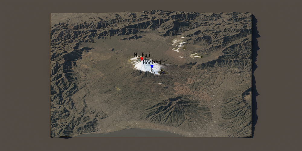
3D visualization of Mount Fuji in Japan.
snakemake --cores 1 -s Snakefile_global
See the code: Snakefile_global
If you want to use this pipeline for a different location and you do not want to use labels, you’ll need to remove the labels from the snakemake pipeline.
Also, see the note about aerial imagery in the previous example.
# Render Parameters File
module_name = "blender_parameters.blender_params_global"

# Import parameters file
import os, sys, importlib
render_params = module_name.replace(".", os.sep) + ".py"
parameters = importlib.import_module(module_name)

# Define the final output
rule all:
    input:
        "phase_2_visualize/out/render_mtfuji.png",
        "fonts/" + parameters.label_font.replace(" ", "_") + ".ttf"

# Download Google Font
rule download_font:
    params:
        label_font = parameters.label_font
    output:
        "fonts/" + parameters.label_font.replace(" ", "_") + ".ttf"
    script:
        "phase_0_fetch/src/download_font.py"

# Creates a multipoint shapefile for labeling
rule create_shapefile:
    params:
        coords = [[35.3606, 138.7274],[35.3438, 138.7522]],
        labels = ["Mt. Fuji", "Hoeizan"],
        pin_colors = [[0.75,0.0,0.0,1.0],[0.0,0.0,0.75,1.0]],
        label_colors = [[0.0,0.0,0.0,1.0],[0.0,0.0,0.0,1.0]],
        crs = "EPSG:4326"
    output:
        shpfile = "phase_0_fetch/out/{name}/labels.shp"
    script:
        "phase_0_fetch/src/make_shpfile.py"

# Make the bounding box
rule make_bounding_box:
    params:
        UL_corner = [35.6, 138.5],
        LR_corner = [35.1, 139.0],
    output:
        extent_shpfile = "phase_0_fetch/out/{name}/extent.shp"
    script:
        "phase_0_fetch/src/make_bounding_box.py"

# Downloads a digital elevation model within extent
rule download_dem:
    params:
        dem_product = parameters.dem_product,
        render_pixels = parameters.res_x * parameters.res_y,
        buffer = parameters.buffer
    input:
        extent_shpfile = "phase_0_fetch/out/{name}/extent.shp"
    output:
        demfile = "phase_0_fetch/out/{name}/dem.tif"
    script:
        "phase_0_fetch/src/download_dem.py"

# Downloads aerial imagery within extent
rule download_aerial:
    params:
        query = {
                "eo:cloud_cover": {"lte": 25},
                "platform":       {"in": ["landsat-8"]}
                },
        start_query = "2021-11-01",
        end_query = "2022-02-01"
    input:
        extent_shpfile = "phase_0_fetch/out/{name}/extent.shp"
    output:
        out_bands = ["phase_0_fetch/out/{name}/" + color + ".tif" for color in ["red", "green", "blue"]]
    script:
        "phase_0_fetch/src/get_imagery.py"

# Creates a grayscale height map and texture map for Blender to render.
# The height map is used to determine how high the landscape should be
# in the render, and the texture map determines the color of the landscape.
rule create_heightmap_texturemap:
    params:
        map_crs = "EPSG:3857",
        buffer = parameters.buffer,
        background_color = parameters.background_color,
        wall_color = parameters.wall_color
    input:
        extent_shpfile = "phase_0_fetch/out/{name}/extent.shp",
        demfile =  "phase_0_fetch/out/{name}/dem.tif",
        aerialfiles =  ["phase_0_fetch/out/{name}/" + color + ".tif" for color in ["red", "green", "blue"]],
        labels_shpfile = "phase_0_fetch/out/{name}/labels.shp"
    output:
        dimensions_file = "phase_1_process/out/{name}/dimensions.npy",
        heightmap_file = "phase_1_process/out/{name}/heightmap.png",
        texturemap_file = "phase_1_process/out/{name}/texturemap.png",
        apronmap_file = "phase_1_process/out/{name}/apronmap.png",
        labels_file = "phase_1_process/out/{name}/labels.csv"
    script:
        "phase_1_process/src/process.py"

# Using the height map and texture map, Blender sets up the scene
# (topography, lighting, and camera) and renders a photorealistic image.
rule render:
    input:
        dimensions_file = "phase_1_process/out/{name}/dimensions.npy",
        heightmap_file = "phase_1_process/out/{name}/heightmap.png",
        texturemap_file = "phase_1_process/out/{name}/texturemap.png",
        apronmap_file = "phase_1_process/out/{name}/apronmap.png",
        labels_file = "phase_1_process/out/{name}/labels.csv",
        blender_params = render_params,
        label_fontfile = "fonts/" + parameters.label_font.replace(" ", "_") + ".ttf"
    output:
        output_file = "phase_2_visualize/out/render_{name}.png"
    shell:
        "Blender -b -P phase_2_visualize/src/render.py -- "
        "{input.blender_params} "
        "{input.dimensions_file} {input.heightmap_file} {input.texturemap_file} {input.apronmap_file} {input.labels_file} "
        "{output.output_file} "
See the parameters: blender_parameters/blender_params_global.py
# For more details about the parameters, please refer to the README in the Github repository:
# https://github.com/DOI-USGS/topo-riv-blender/blob/main/README.md

########## data management ##########
# OpenTopography Products: https://portal.opentopography.org/apidocs/
dem_product = "auto"  # determine automatically
buffer = 0.2  # buffer space around watershed

########## map visualization ##########
background_color = [0.1, 0.1, 0.1, 1.0]
wall_color = [0.1, 0.0667, 0.0333, 1.0]

########## Label Parameters ##########
pin_sides = 4  # sides of pin
pin_height = 0.015  # height of pin
pin_radius1 = 0.0  # bottom of pin
pin_radius2 = 0.00667  # top of pin
pin_label_buffer = 0.05  # space between pin and label
label_scale = 0.035  # size of label
label_font = (
    "Barlow Condensed"  # Specify Google Fonts, Browse here: https://fonts.google.com/
)
shadow_boolean = False  # alllow shadows for the label

########## render hardware ##########
GPU_boolean = False  # if you have a GPU, set this to 1 and this will run faster

########## blender scene ##########
# max dimension on plane
plane_size = 1.0  # meters

########## additional data layers ##########
number_of_layers = 0  # number of additional data layers

########## camera settings ##########
# color management
view_transform = "Filmic"  # 'Standard'
exposure = 0.0  # default is 0
gamma = 0.85  # default is 1

# camera type
camera_type = "orthogonal"  # orthogonal or perspective

# orthogonal
ortho_scale = 1.2  # when using orthogonal scale, increase to "zoom" out

# perspective
focal_length = 50.0  # mm when using perspective camera, increase to zoom in
shift_x = 0.0  # you may need to shift the camera to center the topo in the frame
shift_y = 0.0  # you may need to shift the camera to center the topo in the frame

# camera location
camera_distance = (
    1.0  # meters from the center (maximum horizontal axis is assumed to be 1 meter)
)
camera_tilt = (
    30.0  # degrees from horizontal: 0.0 is profile view, 90.0 is planform view
)
camera_rotation = 180.0  # camera location degrees clockwise from North: 0.0 is North, 90.0 is East, 180.0, is South, and 270.0 is West.

# depth of field
use_depth_of_field = False
dof_distance = camera_distance  # where the focal plane is
f_stop = 100.0  # affects depths of field, lower for a shallow dof, higher for wide dof

########## sun properties ##########
sun_tilt = 20.0  # degrees from horizontal
sun_rotation = 315.0  # degrees clockwise from North
sun_intensity = 0.5  # sun intensity
sun_strength = 1.0  # sun strength

########## landscape representation ###########
min_res = 4000  # minimum resolution of the heightmap, larger value increases detail but takes longer to render
number_of_subdivisions = 2000  # number of subdivisions, larger value increases detail but takes longer to render
exaggeration = "auto"  # vertical exaggeration
displacement_method = "DISPLACEMENT"  # "BOTH" #for more exaggerated shadows

########## render settings ##########
res_x = 3000  # x resolution of the render, larger value increases detail but takes longer to render
res_y = 1500  # y resolution of the render, larger value increases detail but takes longer to render
samples = 10  # number of samples that decides how "good" the render looks, larger value increases detail but takes longer to render
Creating abstract images
You don’t just have to try to make things that look photorealistic.
You can manipulate the topography in any way.
Here, we create a contour map from the original topography to give the landscape a “terraced” effect.
We also specify a color map in matplotlib to create a custom color gradient across the elevation values.
Last, this workflow showcases some of the camera effects you can use within Blender.
Here, we use a depth-of-field effect that causes the landscape to look blurry up close and far away.
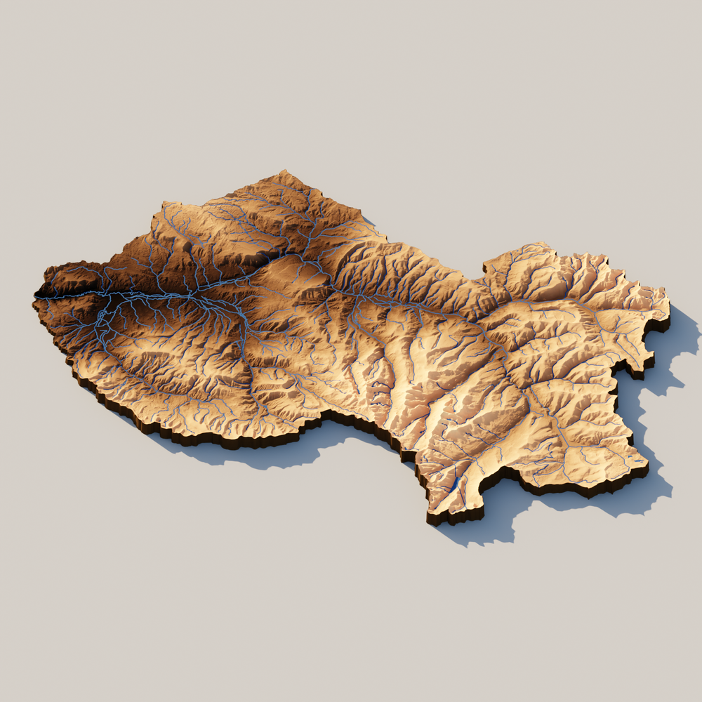
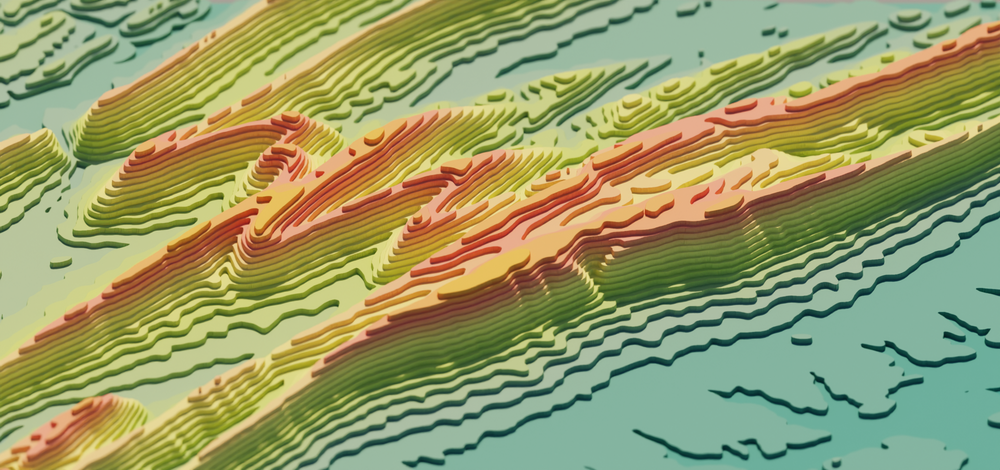
3D visualization of the Columbia River in Oregon and Washington, USA.
snakemake --cores 1 -s Snakefile_contour
See the code: Snakefile_contour
# Render Parameters File
module_name = "blender_parameters.blender_params_contour"

# Import parameters file
import os, sys, importlib
render_params = module_name.replace(".", os.sep) + ".py"
parameters = importlib.import_module(module_name)

# Define the final output
rule all:
    input:
        "phase_2_visualize/out/render_columbiariver.png",

# Make the bounding box
rule make_bounding_box:
    params:
        UL_corner = [45.85, -121.65],
        LR_corner = [45.50, -121.19],
    output:
        extent_shpfile = "phase_0_fetch/out/{name}/extent.shp"
    script:
        "phase_0_fetch/src/make_bounding_box.py"

# Downloads a digital elevation model within extent
rule download_dem:
    params:
        dem_product = parameters.dem_product,
        buffer = parameters.buffer
    input:
        extent_shpfile = "phase_0_fetch/out/{name}/extent.shp"
    output:
        demfile = "phase_0_fetch/out/{name}/dem.tif"
    script:
        "phase_0_fetch/src/download_dem.py"

# Creates a grayscale height map and texture map for Blender to render.
# The height map is used to determine how high the landscape should be
# in the render, and the texture map determines the color of the landscape.
rule create_heightmap_texturemap:
    params:
        map_crs = "EPSG:3857",
        mask_boolean = False,
        contour_boolean = True,
        topo_cmap = parameters.topo_cmap,
        topo_cstops = parameters.topo_cstops,
        buffer = parameters.buffer
    input:
        extent_shpfile = "phase_0_fetch/out/{name}/extent.shp",
        demfile =  "phase_0_fetch/out/{name}/dem.tif",
    output:
        dimensions_file = "phase_1_process/out/{name}/dimensions.npy",
        heightmap_file = "phase_1_process/out/{name}/heightmap.png",
        texturemap_file = "phase_1_process/out/{name}/texturemap.png",
        apronmap_file = "phase_1_process/out/{name}/apronmap.png"
    script:
        "phase_1_process/src/process.py"

# Using the height map and texture map, Blender sets up the scene
# (topography, lighting, and camera) and renders a photorealistic image.
rule render:
    input:
        dimensions_file = "phase_1_process/out/{name}/dimensions.npy",
        heightmap_file = "phase_1_process/out/{name}/heightmap.png",
        texturemap_file = "phase_1_process/out/{name}/texturemap.png",
        apronmap_file = "phase_1_process/out/{name}/apronmap.png",
        blender_params = render_params
    output:
        output_file = "phase_2_visualize/out/render_{name}.png"
    shell:
        "Blender -b -P phase_2_visualize/src/render.py -- "
        "{input.blender_params} "
        "{input.dimensions_file} {input.heightmap_file} {input.texturemap_file} {input.apronmap_file} NULL "
        "{output.output_file} "
See the parameters: blender_parameters/blender_params_contour.py
# For more details about the parameters, please refer to the README in the Github repository:
# https://github.com/DOI-USGS/topo-riv-blender/blob/main/README.md

########## data management ##########
# OpenTopography Products: https://portal.opentopography.org/apidocs/
dem_product = "USGS10m"  # usgs 10m
buffer = 0.2  # buffer space around watershed

########## map visualization ##########

# topography colormap
topo_cmap = "custom"
topo_cstops = [
    [70, 140, 131],
    [134, 166, 144],
    [185, 202, 110],
    [237, 224, 132],
    [242, 140, 119],
    [242, 177, 71],
]

########## render hardware ##########
GPU_boolean = False  # if you have a GPU, set this to 1 and this will run faster

########## blender scene ##########
# max dimension of plane
plane_size = 1.0  # meters

########## additional data layers ##########
number_of_layers = 0  # number of additional data layers

########## camera settings ##########
# color management
view_transform = "Filmic"  # 'Standard'
exposure = -2.0  #'default is 0
gamma = 0.5  # default is 1

# camera type
camera_type = "orthogonal"  # orthogonal or perspective

# orthogonal
ortho_scale = 0.8  # when using orthogonal scale, increase to "zoom" out

# perspective
focal_length = 50.0  # mm when using perspective camera, increase to zoom in
shift_x = 0.0  # you may need to shift the camera to center the topo in the frame
shift_y = 0.05  # you may need to shift the camera to center the topo in the frame

# camera location
camera_distance = (
    1.0  # meters from the center (maximum horizontal axis is assumed to be 1 meter)
)
camera_tilt = (
    30.0  # degrees from horizontal: 0.0 is profile view, 90.0 is planform view
)
camera_rotation = 180.0  # camera location degrees clockwise from North: 0.0 is North, 90.0 is East, 180.0, is South, and 270.0 is West.

# depth of field
use_depth_of_field = True
dof_distance = camera_distance  # where the focal plane is
f_stop = 100.0  # affects depths of field, lower for a shallow dof, higher for wide dof

########## sun properties ##########
sun_tilt = 45.0  # degrees from horizontal
sun_rotation = 0.0  # degrees clockwise from North
sun_intensity = 0.5  # sun intensity
sun_strength = 1.0  # sun strength

########## landscape representation ###########
min_res = 2000  # minimum resolution of the height map, larger value increases detail but takes longer to render
number_of_subdivisions = 2000  # number of subdivisions, larger value increases detail but takes longer to render
exaggeration = 5.0  # vertical exaggeration
displacement_method = "DISPLACEMENT"  # "BOTH" #for more exaggerated shadows

########## render settings ##########
res_x = 2000  # x resolution of the render, larger value increases detail but takes longer to render
res_y = 940  # y resolution of the render, larger value increases detail but takes longer to render
samples = 10  # number of samples that decides how "good" the render looks, larger value increases detail but takes longer to render
Adding an ocean/lake layer
The default workflow uses a single layer, the topography.
However, the functions in topo-riv-blender allow rendering of multiple layers.
In this workflow, we include a water layer that has a transparent blue color.
We set this layer as a flat plane at the average lake level to differentiate between the topography and bathymetry.
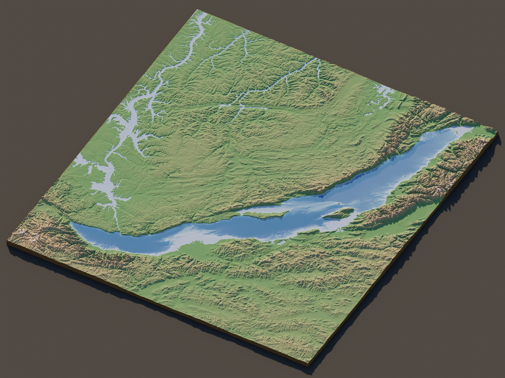
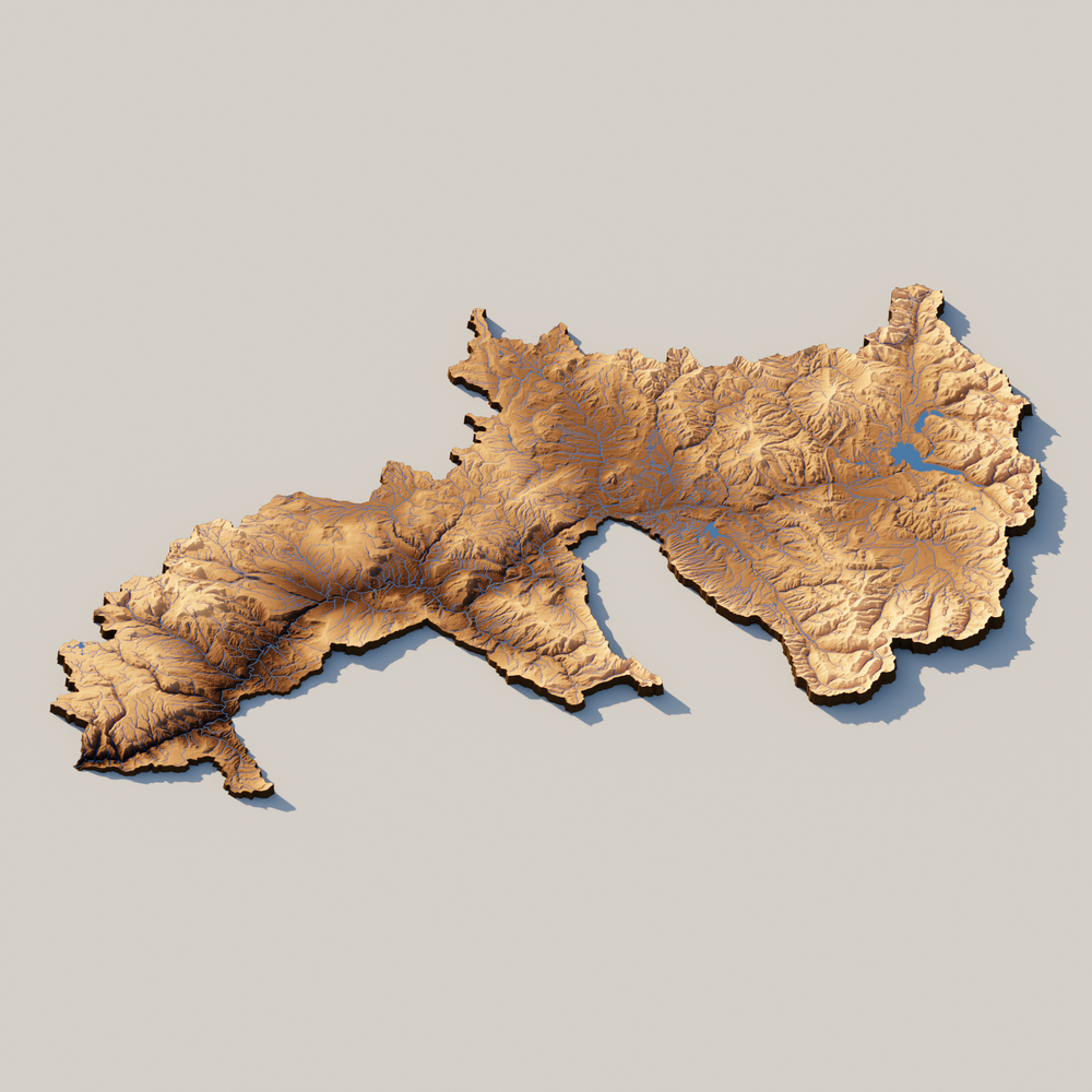
3D visualization of Lake Baikal in Siberia, Russia.
snakemake --cores 1 -s Snakefile_lake
See the code: Snakefile_lake
# Render Parameters File
module_name = "blender_parameters.blender_params_lake"

# Import parameters file
import os, sys, importlib
render_params = module_name.replace(".", os.sep) + ".py"
parameters = importlib.import_module(module_name)

# Define the final output
rule all:
    input:
        "phase_2_visualize/out/render_lakebaikal.png",

# Make the bounding box
rule make_bounding_box:
    params:
        UL_corner = [56.03371860720012, 102.75351112656995],
        LR_corner = [50.919371945323256, 110.61494439816751],
    output:
        extent_shpfile = "phase_0_fetch/out/{name}/extent.shp"
    script:
        "phase_0_fetch/src/make_bounding_box.py"

# Downloads a digital elevation model within extent
rule download_dem:
    params:
        dem_product = parameters.dem_product,
        render_pixels = parameters.res_x * parameters.res_y,
        buffer = parameters.buffer
    input:
        extent_shpfile = "phase_0_fetch/out/{name}/extent.shp"
    output:
        demfile = "phase_0_fetch/out/{name}/dem.tif"
    script:
        "phase_0_fetch/src/download_dem.py"

# Creates a grayscale height map and texture map for Blender to render.
# The height map is used to determine how high the landscape should be
# in the render, and the texture map determines the color of the landscape.
rule create_heightmap_texturemap:
    params:
        map_crs = "EPSG:3857",
        buffer = parameters.buffer,
        topo_cmap = parameters.topo_cmap,
        topo_cstops = parameters.topo_cstops,
        topo_nstops = parameters.topo_nstops,
        oceanfloor_cmap = parameters.oceanfloor_cmap,
        ocean_elevation = parameters.ocean_elevation,
        background_color = parameters.background_color,
        wall_color = parameters.wall_color,
        ocean_boolean = True
    input:
        extent_shpfile = "phase_0_fetch/out/{name}/extent.shp",
        demfile =  "phase_0_fetch/out/{name}/dem.tif",
    output:
        dimensions_file = "phase_1_process/out/{name}/dimensions.npy",
        heightmap_file = "phase_1_process/out/{name}/heightmap.png",
        texturemap_file = "phase_1_process/out/{name}/texturemap.png",
        heightmap_layerfiles = ["phase_1_process/out/{name}/heightmap_L0.png"],
        texturemap_layerfiles = ["phase_1_process/out/{name}/texturemap_L0.png"],
        apronmap_file = "phase_1_process/out/{name}/apronmap.png"
    script:
        "phase_1_process/src/process.py"

# Using the height map and texture map, Blender sets up the scene
# (topography, lighting, and camera) and renders a photorealistic image.
rule render:
    input:
        dimensions_file = "phase_1_process/out/{name}/dimensions.npy",
        heightmap_file = "phase_1_process/out/{name}/heightmap.png",
        texturemap_file = "phase_1_process/out/{name}/texturemap.png",
        heightmap_layerfiles = ["phase_1_process/out/{name}/heightmap_L0.png"],
        texturemap_layerfiles = ["phase_1_process/out/{name}/texturemap_L0.png"],
        apronmap_file = "phase_1_process/out/{name}/apronmap.png",
        blender_params = render_params
    output:
        output_file = "phase_2_visualize/out/render_{name}.png"
    shell:
        "Blender -b -P phase_2_visualize/src/render.py -- "
        "{input.blender_params} "
        "{input.dimensions_file} {input.heightmap_file} {input.texturemap_file} {input.apronmap_file} NULL "
        "{output.output_file} "
See the parameters: blender_parameters/blender_params_lake.py
When using this pipeline for your own use make sure to adjust the ocean_elevation, otherwise everything might be underwater! For Lake Baikal, I just googled it’s general water surface elevation.
# For more details about the parameters, please refer to the README in the Github repository:
# https://github.com/DOI-USGS/topo-riv-blender/blob/main/README.md

########## data management ##########
# OpenTopography Products: https://portal.opentopography.org/apidocs/
dem_product = "SRTM15Plus"  # "GEBCOIceTopo"  # determine automatically
buffer = 0.2  # buffer space around watershed

########## map visualization ##########
background_color = [0.1, 0.1, 0.1, 1.0]
wall_color = [0.2, 0.133, 0.0667, 1.0]

# topography colormap
topo_cmap = "custom"
topo_cstops = [[42, 64, 42], [88, 70, 56], [200, 200, 200]]
topo_nstops = [0, 200, 256]

# "ocean" parameters
oceanfloor_cmap = "bone"
ocean_elevation = 455.5  # m

########## render hardware ##########
GPU_boolean = False  # if you have a GPU, set this to 1 and this will run faster

########## blender scene ##########
# max dimension on plane
plane_size = 1.0  # meters

########## additional data layers ##########
number_of_layers = 1  # number of additional data layers
layers_alpha = [0.75]

########## camera settings ##########
# color management
view_transform = "Filmic"  # 'Standard'
exposure = 0.0  # default is 0
gamma = 0.85  # default is 1

# camera type
camera_type = "orthogonal"  # orthogonal or perspective

# orthogonal
ortho_scale = 1.3  # when using orthogonal scale, increase to "zoom" out

# perspective
focal_length = 50.0  # mm when using perspective camera, increase to zoom in
shift_x = 0.0  # you may need to shift the camera to center the topo in the frame
shift_y = 0.0  # you may need to shift the camera to center the topo in the frame

# camera location
camera_distance = (
    1.0  # meters from the center (maximum horizontal axis is assumed to be 1 meter)
)
camera_tilt = (
    45.0  # degrees from horizontal: 0.0 is profile view, 90.0 is planform view
)
camera_rotation = 150.0  # camera location degrees clockwise from North: 0.0 is North, 90.0 is East, 180.0, is South, and 270.0 is West.

# depth of field
use_depth_of_field = False
dof_distance = camera_distance  # where the focal plane is
f_stop = 100.0  # affects depths of field, lower for a shallow dof, higher for wide dof

########## sun properties ##########
sun_tilt = 20.0  # degrees from horizontal
sun_rotation = 315.0  # degrees clockwise from North
sun_intensity = 0.5  # sun intensity
sun_strength = 1.0  # sun strength

########## landscape representation ###########
min_res = 4000  # minimum resolution of the heightmap, larger value increases detail but takes longer to render
number_of_subdivisions = 2000  # number of subdivisions, larger value increases detail but takes longer to render
exaggeration = 5.0  # vertical exaggeration
displacement_method = "DISPLACEMENT"  # "BOTH" #for more exaggerated shadows

########## render settings ##########
res_x = 2000  # x resolution of the render, larger value increases detail but takes longer to render
res_y = 1500  # y resolution of the render, larger value increases detail but takes longer to render
samples = 10  # number of samples that decides how "good" the render looks, larger value increases detail but takes longer to render
Creating the thumbnail for this blog
Did you click this blog because the thumbnail on the WDFN blog gallery looked cool? If you did, thanks! I created this thumbnail to represent this geospatial data pipeline. I hope you can use this to make other attractive thumbnails to get people to click on your work!
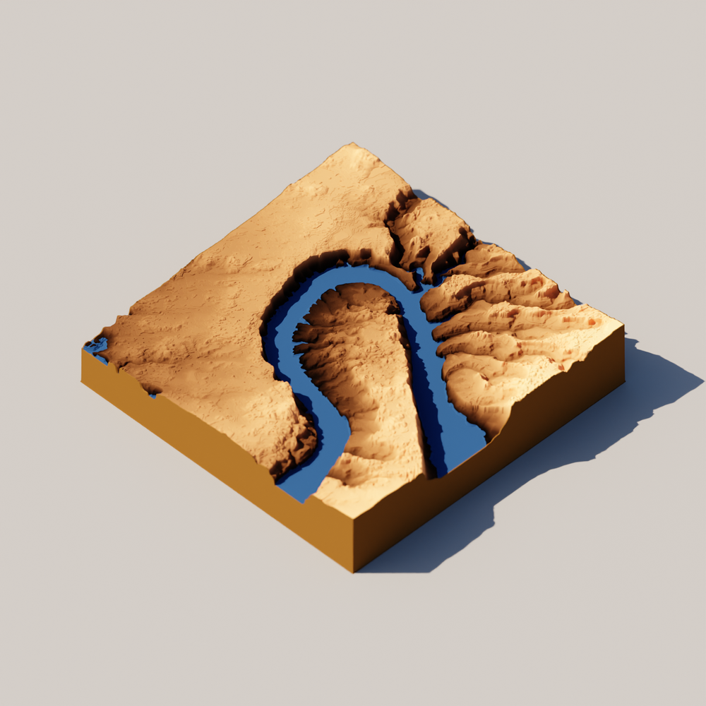
3D visualization of the Colorado River in Southern Utah, USA.
snakemake --cores 1 -s Snakefile_thumbnail
See the code: Snakefile_thumbnail
# Render Parameters File
module_name = "blender_parameters.blender_params_thumbnail"

# Import parameters file
import os, sys, importlib
render_params = module_name.replace(".", os.sep) + ".py"
parameters = importlib.import_module(module_name)

square = 0.06
aspect = 1.25755052918
UL_corner_specify = [37.36615071600088, -110.8944504506659]

# Define the final output
rule all:
    input:
        "phase_2_visualize/out/render_thumbnail.png",

# Make the bounding box
rule make_bounding_box:
    params:
        UL_corner =[UL_corner_specify[0], UL_corner_specify[1]],
        LR_corner = [UL_corner_specify[0]-square, UL_corner_specify[1]+square*aspect],
    output:
        extent_shpfile = "phase_0_fetch/out/{name}/extent.shp"
    script:
        "phase_0_fetch/src/make_bounding_box.py"

# Downloads a digital elevation model within extent
rule download_dem:
    params:
        dem_product = parameters.dem_product,
        buffer = parameters.buffer
    input:
        extent_shpfile = "phase_0_fetch/out/{name}/extent.shp"
    output:
        demfile = "phase_0_fetch/out/{name}/dem.tif"
    script:
        "phase_0_fetch/src/download_dem.py"

# Downloads NHD waterbody data within extent
rule get_nhd_wb:
    params:
        nhd_type = parameters.nhd_waterbody,
        render_pixels = parameters.res_x * parameters.res_y
    input:
        extent_shpfile = "phase_0_fetch/out/{name}/extent.shp"
    output:
        nhd_shpfile = "phase_0_fetch/out/{name}/waterbody.shp"
    script:
        "phase_0_fetch/src/get_nhd.py"

# Creates a grayscale height map and texture map for Blender to render.
# The height map is used to determine how high the landscape should be
# in the render, and the texture map determines the color of the landscape.
rule create_heightmap_texturemap:
    params:
        map_crs = "EPSG:3857",
        topo_cmap = parameters.topo_cmap,
        buffer = parameters.buffer,
        wall_thickness = 4.0,
        wall_color = [0.4, 0.266, 0.133, 1.0],
        background_color = [0.5, 0.5, 0.5, 1.0],
        custom_min_dem = 600.0
    input:
        extent_shpfile = "phase_0_fetch/out/{name}/extent.shp",
        demfile =  "phase_0_fetch/out/{name}/dem.tif",
        waterbody_shpfile = "phase_0_fetch/out/{name}/waterbody.shp"
    output:
        dimensions_file = "phase_1_process/out/{name}/dimensions.npy",
        heightmap_file = "phase_1_process/out/{name}/heightmap.png",
        texturemap_file = "phase_1_process/out/{name}/texturemap.png",
        apronmap_file = "phase_1_process/out/{name}/apronmap.png"
    script:
        "phase_1_process/src/process.py"

# Using the height map and texture map, Blender sets up the scene
# (topography, lighting, and camera) and renders a photorealistic image.
rule render:
    input:
        dimensions_file = "phase_1_process/out/{name}/dimensions.npy",
        heightmap_file = "phase_1_process/out/{name}/heightmap.png",
        texturemap_file = "phase_1_process/out/{name}/texturemap.png",
        apronmap_file = "phase_1_process/out/{name}/apronmap.png",
        blender_params = render_params
    output:
        output_file = "phase_2_visualize/out/render_{name}.png"
    shell:
        "Blender -b -P phase_2_visualize/src/render.py -- "
        "{input.blender_params} "
        "{input.dimensions_file} {input.heightmap_file} {input.texturemap_file} {input.apronmap_file} NULL "
        "{output.output_file} "
See the parameters: blender_parameters/blender_params_thumbnail.py
# For more details about the parameters, please refer to the README in the Github repository:
# https://github.com/DOI-USGS/topo-riv-blender/blob/main/README.md

########## data management ##########
# OpenTopography Products: https://portal.opentopography.org/apidocs/
dem_product = "USGS10m"  # usgs 10m
buffer = 0.2  # buffer space around watershed
# NHD products
nhd_flowline = "flowline_auto"  # use auto, mr, or hr
nhd_waterbody = "waterbody_hr"  # use auto, mr, or hr

########## map visualization ##########

# topography colormap
topo_cmap = "copper"

########## render hardware ##########
GPU_boolean = False  # if you have a GPU, set this to 1 and this will run faster

########## blender scene ##########
# max dimension of plane
plane_size = 1.0  # meters

########## additional data layers ##########
number_of_layers = 0  # number of additional data layers

########## camera settings ##########
# color management
view_transform = "Filmic"  # 'Standard'
exposure = -0.75  #'default is 0
gamma = 0.5  # default is 1

# camera type
camera_type = "orthogonal"  # orthogonal or perspective

# orthogonal
ortho_scale = 1.8  # when using orthogonal scale, increase to "zoom" out

# perspective
focal_length = 50.0  # mm when using perspective camera, increase to zoom in
shift_x = 0.0  # you may need to shift the camera to center the topo in the frame
shift_y = 0.04  # you may need to shift the camera to center the topo in the frame

# camera location
camera_distance = (
    1.0  # meters from the center (maximum horizontal axis is assumed to be 1 meter)
)
camera_tilt = (
    45.0  # degrees from horizontal: 0.0 is profile view, 90.0 is planform view
)
camera_rotation = 135.0  # camera location degrees clockwise from North: 0.0 is North, 90.0 is East, 180.0, is South, and 270.0 is West.

# depth of field
use_depth_of_field = True
dof_distance = camera_distance  # where the focal plane is
f_stop = 100.0  # affects depths of field, lower for a shallow dof, higher for wide dof

########## sun properties ##########
sun_tilt = 45.0  # degrees from horizontal
sun_rotation = 225.0  # degrees clockwise from North
sun_intensity = 0.5  # sun intensity
sun_strength = 1.0  # sun strength

########## landscape representation ###########
min_res = 2000  # minimum resolution of the height map, larger value increases detail but takes longer to render
number_of_subdivisions = 2000  # number of subdivisions, larger value increases detail but takes longer to render
exaggeration = 2.0  # vertical exaggeration
displacement_method = "DISPLACEMENT"  # "BOTH" #for more exaggerated shadows

########## render settings ##########
res_x = 1500  # x resolution of the render, larger value increases detail but takes longer to render
res_y = 1500  # y resolution of the render, larger value increases detail but takes longer to render
samples = 10  # number of samples that decides how "good" the render looks, larger value increases detail but takes longer to render
Apply the example workflows to a different location!
If you like these example workflows, you can easily adjust them to create images of different locations.
In contrast to the default Snakefile, these example workflows require the user to specify a bounding box instead of a HUC ID.
If you want to change the location or add/remove data components, you will want to modify the Snakefiles.
Inside the different Snakefiles (e.g., Snakefile_contour), look for the following parameters:
UL_corner = [45.85, -121.65],
LR_corner = [45.50, -121.19],
You will see two sets of coordinates (latitude, longitude in decimal degrees).
UL_corner stands for the upper left corner and LR_corner stands for the lower right corner.
A simple way to find the location is by using Google Maps
.
Right-click a point, copy the coordinates in the context menu, and paste them between the brackets.
For example, we can change the bounding box to the following coordinates:
UL_corner = [40.33, -77.75],
LR_corner = [40.11, -77.43],
These coordinates correspond to an area in the Tuscarora State Forest.
Next you’ll want to modify the output filename in rule all in the Snakefile.
Before:
rule all:
    input:
        "phase_2_visualize/out/render_columbiariver.png",
After:
rule all:
    input:
        "phase_2_visualize/out/render_tuscarora.png",
Rerun the snakemake command, and the workflow will make an image for your new location.
3D visualization of Tuscarora State Forest in Central Pennsylvania, USA.
Takeaways
topo-riv-blender is a reproducible Python workflow that takes geospatial data (topographic, hydrographic, and imagery) and processes it to be rendered into 3D images using Blender.
The repository houses flexible workflows that you can customize to change the look and location of the image.
We also provide these workflows to serve as templates for creating your own scientific or artistic visualizations.
More information to help you get started can be found in the README.md
file.
We hope this has inspired you to use Blender and look forward to seeing what you make!
Additional resources
Below are some of the Python packages and datasets that we leverage to make this pipeline possible.
- HyRiver
is a useful suite of
Pythonpackages that we use to fetch river, waterbody, and watershed shape files. - OpenTopography is an NSF-EAR funded data facility that provides open and free access to regional and global (10-90m resolution) digital elevation models.
- BMI Topography
is a
Pythonlibrary that we use to fetch the different topography products from OpenTopography. - Planetary Computer Data Catalog houses a diverse collection of remote sensing products that you can pull with the STAC API.
- Blender Python API provides useful documentation that allows you to programmatically create Blender scenes and visualizations.
Acknowledgments
The genesis of this workflow was made possible through collaboration with the USGS 3DHP team. This work was supported by funding from the USGS Community for Data Integration (CDI). Award link: 2025 Community for Data Integration (CDI) award .
Disclaimer
Any use of trade, firm, or product names is for descriptive purposes only and does not imply endorsement by the U.S. Government.
Categories:
Related Posts
Large, parallel deep learning experiments using Snakemake
April 19, 2022
A paper we wrote was recently published! In the paper we had to run and evaluate many DL model runs. This post is all about how we automated these model runs and executed them in parallel using the workflow management software, Snakemake .