
Extracting the grammar of U.S. stream names
Building a reproducible system for identifying the generic feature words from stream names using R.
What's on this page
English is the official language and authoritative version of all federal information.
Extracting a stream’s feature
The names of streams (hydronyms ) contain, hidden within them, the power to show us the linguistic patterns within the United States. In the United States, stream names tend to follow a binomial structure: a specific name (“Moose,” “Columbia,” “Snake”) paired with a generic feature word (“creek,” “river,” “fork,” “bayou”). The specific portion is endlessly variable, but the generic part is surprisingly stable. In fact, if you look at stream names across the country, the diversity of generic terms is relatively small, but shaped by centuries of hydrologic realities, settlement history, and local tradition.
This post focuses entirely on that second component: extracting the correct generic feature word from every stream name in the Geographic Names Information System (GNIS) database, the U.S. Geological Survey’s official repository of place names. This step is essential for the visualizations introduced in A map that glows with the vocabulary of water .
At first glance, finding the feature word sounds simple: take the last word, right? “Moose Creek.” Done. That works… sometimes. In practice, stream names are wildly inconsistent. The feature might be the first word, the last word, or hiding in the middle. Some names include adjectives, articles, or multi-word constructions. Others come from languages besides English: Spanish, French, Dutch, Indigenous languages, or hybrid forms. Consider a few examples:
- Fourche LaFave River
- North Fork White River
- Rio Puerco
- Big Bogue Homa
- Toothaker Brook Number One
Each follows a different grammatical logic. Our task is to build a workflow flexible enough to handle all (or at least most) of them (about 220,000 names in total) without resorting to manual editing or case-by-case exceptions.
The goal of this post is to walk through a robust, reproducible system for identifying the feature word, using a blend of linguistic heuristics, frequency analysis, and rule-based extraction. By the end, we’ll have a nice and tidy table of streams, their coordinates, and the correctly extracted feature. This dataset will unlock the cultural and historical mapping done in the A map that glows with the vocabulary of water . Like this:
Understanding the problem
The Geographic Names Information System (GNIS) is the official repository of domestic geographic names data in the United States, maintained by the U.S. Geological Survey (USGS) in cooperation with the interagency U.S. Board on Geographic Names (BGN). Originally developed in the 1970s to support standardization of geographic names across federal agencies, GNIS contains detailed information on over two million physical and cultural geographic features, including populated places, summits, lakes, and streams. GNIS provides standardized names, feature types, geographic coordinates, elevation, and some naming information.
The BGN oversees the standardization of geographic names used by the federal government, which are cataloged in GNIS. Originally established in 1890 and formalized by public law in 1947, the BGN ensures that geographic names are applied consistently across federal maps, publications, and databases. It reviews proposals for new names or name changes and adjudicates naming disputes. The BGN’s decisions directly inform updates to the GNIS, making it a critical authority in the stewardship of geographic nomenclature.
GNIS data is available in a number of ways. There is an interactive Domestic Names Search Tool , a REST ArcGIS API , and direct file downloads from the The National Map Staged Products Directory . We will use the latter to download the entire national Domestic Names dataset.
Before we start downloading and manipulating the data, we first need to get the R coding environment set up. This should be pretty easy; we just need to install our packages and set our encoding locale. This will help ensure we are working with the same set of tools and that we can handle names with characters that aren’t available in every encoding (like ñ).
# Install necessary packages
install.packages(c(
  "sf",      # For reading and handling spatial points
  "dplyr",   # For manipulating data frames
  "stringr", # For string manipulation
  "readr"    # For writing our data
))

# Attach packages that we'll really rely on
library(sf)
library(dplyr)
library(stringr)
library(readr)
There are a few ways to download the data, but we’ll use the approach that I find both efficient and interesting: downloading a GeoPackage (GPKG) directly. A GPKG is a spatial file format that can store multiple layers of spatial data. The benefit of this method is that we can leverage powerful utilities designed for spatial datasets, allowing us to retrieve only the subset of data we need without first downloading and unzipping files on our computer. Instead, we access it through the URL and the data is transferred into our memory directly (See sf::st_read()
and GDAL Virtual File Systems
for more information). No more separate downloading and unzipping steps! Even better, we can use SQL statements (which tend to be fairly intuitive because much of the tidyverse syntax is based on SQL terminology) to filter the data and do other processing steps before it gets fully loaded into our memory (See sf::st_read()
and OGR SQL dialect
for more information). This means that even though the full dataset is quite large (around 400 MB), we can extract only the portion we need without loading the entire file. Pretty slick! The URL structure and SQL queries might look unusual at first, so I’ll break them down into pieces.
# Construct DSN to access GNIS data directly from API
gnis_gpkg_url <- paste0(
  "/vsizip/vsicurl/", # Fetch file from URL and then access data within zip file
  "https://prd-tnm.s3.amazonaws.com/StagedProducts/GeographicNames/FullModel/", # URL
  "Gazetteer_National_GDB.zip/Gazetteer_National_GDB.gdb" # File
)

# Build SQL statements to filter, select, and rename before loading into memory
gnis_query <- paste0(
  # Return only feature_name (rename to stream_name), prim_lat_dec, prim_long_dec
  "SELECT feature_name AS stream_name, prim_lat_dec, prim_long_dec ",
  # From the Domestic Names layer
  "FROM DomesticNames ",
  # For rows with the Stream feature class and
  "WHERE feature_class = 'Stream' AND state_name IN ('",
  paste(state.name[!state.name %in% c("Alaska", "Hawaii")], collapse = "', '"),
  "')"
)

# Read in queried data from URL
# This will take a little bit, maybe about a minute
stream_df <- sf::st_read(
  dsn = gnis_gpkg_url,
  query = gnis_query,
  as_tibble = TRUE
) |>
  # This data has line points all along the streams that we don't need
  st_drop_geometry()

stream_df
#> # A tibble: 220,317 × 3
#>    stream_name       prim_lat_dec prim_long_dec
#>  * <chr>                    <dbl>         <dbl>
#>  1 Missouri River            38.8         -90.1
#>  2 Mississippi River         29.2         -89.3
#>  3 Rio Grande                26.0         -97.1
#>  4 Arkansas River            33.8         -91.1
#>  5 Snake River               46.2        -119.
#>  6 Ohio River                37.0         -89.1
#>  7 Canadian River            35.5         -95.0
#>  8 Columbia River            46.2        -124.
#>  9 Red River                 31.0         -91.7
#> 10 Yellowstone River         48.0        -104.
#> # ℹ 220,307 more rows
#> # ℹ Use `print(n = ...)` to see more rows
This takes a little bit of time. It is dependent of the individual computer and internet connection, but on my laptop it takes about 30 seconds to run all that. But whoa, that was a lot of heavy lifting! We were able to skip a several steps and loading unnecessary data into our memory. Now let’s talk about the logic behind our analysis before we start building our workflow.
Why GNIS names are messy
The stream names cataloged in GNIS are rich, fascinating, and utterly inconsistent. They come with stylistic quirks accumulated over centuries of naming practices and bureaucratic edits. Some common issues include:
- Mixed capitalization and inconsistent formatting
- Spanish words without tildes (“La Canada” even when the intended form is “La Cañada”)
- Trailing descriptors, including “(historical),” “(not official),” or numbered labels (“Number Two”)
- Adjectives and articles that obscure the underlying feature term (that is to say, Stop words )
- Non-English influences, which can change the location of the generic word within the stream name
Because the BGN and GNIS prioritize consistency and accuracy of use in official labels rather than enforcing some grammatical structure, the underlying linguistic patterns of stream names remain uneven. For the purposes of analysis or mapping, that messiness has to be untangled.
ℹ️ A quick aside on accents and diacritical marks
One notable aspect of inconsistencies within GNIS stream names is the use of accents and other diacritics. For example, in GNIS the French rivière and the Spanish ciénega are both cataloged without marks as riviere and cienega; however, the ñ is retained in cañada. Per Policy VI of the BGN's Domestic Geographic Names Policies, diacritic marks are allowed but often omitted because many stream names from "non-English languages have been assimilated into English language usage and lack the diacritics from the original spelling." These marks are most often included in the spelling "if their omission would result in a significant change in pronunciation or meaning." So in the examples given, we can infer that the BGN decided that the accented vowels didn't substantially impact the pronunciation or meaning in riviere and cienega, but it did impact cañada.
What counts as a “feature word”
For this project, the feature word is the generic hydrographic classifier: the term that identifies what kind of waterway it is. It is the word that remains meaningful across contexts, even though the specific portion of the name may change. Some (most) stream names are pretty easy to parse and have just a single feature word in the name. Others are in unconventional word orders or have multiple generic names where you may have to parse the syntax to identify the most relevant feature word. For example:
- Corn Creek Wash (This is the Wash specified by “Corn Creek”", not the Creek specified as both “Corn”" and “Wash”")
- Star Arm Branch
- Left Fork Hurricane Creek (Similarly, this is the Fork of “Hurricane Creek” not the Creek of “Left Fork Hurricane”)
- Old Channel Bayou De View
These words act like cultural markers that allow patterns in their spatial distribution to be observed because there are relatively few compared to the infinite possibilities of the specific name.
The overall strategy
The workflow proceeds in two major stages:
- First-pass rules: Detect strong, highly patterned features like branching terms (e.g., “fork,” “run,” “branch”) or Latin language (Spanish/French) terms (e.g., “rio,” “arroyo,” “riviere,” “estero”), and remove misleading prefixes and suffixes when necessary.
- Second-pass refinement: Build a frequency-ranked vocabulary of feature words and use it to resolve ambiguous names, choosing the most likely candidate based on how often it appears across the national dataset.
This two-stage approach strikes a balance between linguistic intuition and data-driven regularization. The first stage captures the grammatical logic and the second stage cleans up the noise.
Preprocessing: Normalizing Names Before Extraction
Nearly every downstream step relies on pattern matching: prefix removal, branching term detection, first/last word extraction, and frequency ranking. If the text is not standardized upfront, every “maybe” in the data multiplies the possible error rate of the analysis. So before we can extract anything, the names need to be standardized. Normalization includes:
- Converting everything to lowercase
- Removing GNIS suffixes “(historical)” or “(not official)”
- Stripping numeric qualifiers (Number Two or Number 14)
- Removing extra whitespace
# Perform initial name normalization
stream_df_norm <- stream_df |>
  mutate(
    # Keep the original stream name
    stream_name_orig = stream_name,
    # Normalize stream name
    stream_name = stream_name |>
      str_to_lower() |> # Covert to lower case
      # Remove common suffixes: "(historical), (not official), and "Number __"
      stringr::str_remove("(\\(historical\\)|\\(not official\\))$") |>
      stringr::str_remove("number(\\s(\\d+|one|two|three|eight|fourteen))?$") |>
      stringr::str_squish() # Remove extra whitespace
  )
Normalizing here prevents false negatives later, especially when searching for multi-word patterns or relying on frequency comparisons.
Standardizing known orthographic inconsistencies
Beyond this normalization, some names require special handling. An example that I bumped into was: La Canada → La Cañada. This distinction matters because Cañada is a common generic feature word in some Spanish-influenced regions (roughly translating to gully, stream, or glen), whereas Canada is typically a specific name with no connection to stream morphology (like the country). Without standardizing these cases, the workflow would silently miss major cultural-linguistic patterns.
# Replace common spelling inconsistency (la canada -> la cañada)
stream_df_norm <- stream_df_norm |>
  mutate(stream_name = str_replace(stream_name, "la canada", "la cañada"))
We want to make sure we do this before we do future tasks like removing Spanish articles (including “la”) because that is our best bet in identifying where “canada” should be “cañada”.
Classifying names into rule systems
You can’t meaningfully extract a feature without knowing the grammar of the name. English, Spanish, French, Creole, and branching systems place the important word in different positions. The rule-class assignment is what tells the workflow where to look for the correct feature. There are two rules that we’ll implement here which carry strong grammatical patterns that will complicate our identification of our feature term if unaddressed: (1) Latin-language influence and (2) named branches of streams.
Latin-root hydronyms
Many stream names across the Southwest, Gulf Coast, and parts of the East exhibit Spanish, French, or Creole grammatical structures. These systems often place articles or adjectives before the feature word, producing sequences like:
- El Arroyo Seco
- La Cañada Verde
- La Fourche du Tchefuncte
To properly extract the feature, these prefixes must be stripped away. Words like “el,” “la,” “los,” “las” are never the generic component and can muddy the waters. Removing them restores the internal structure and prevents misclassification.
Another phenomena is the mixing of English adjectives and non-English grammatical structures, which is especially prevalent in the names of Bayous. For example:
- Little Bayou Pierre
- West Bayou Grand Marais
- Big Bayou Pigeon
Here, in a pattern somewhat similar to the Spanish/French articles, the adjectives precede the generic name and then the specific name follows.
From here on, I’ll use the term “Latin” to refer to the broad family of naming traditions derived from Spanish and French settlement histories.
Branching hydronyms
Another common system includes branching terms such as fork, run, branch, prong, and fourche. These often appear with directional adjectives:
- North Fork…
- West Prong…
- Middle Run…
In these constructions, the feature is the second word, not the first or last. If you simply extract the last word, you get “river” instead of “fork” in names like North Fork of the Clearwater River. But the more specific and meaningful feature (for our purposes) is “fork.” Detecting and prioritizing this structure is important if we want to compare the generic hydronym across the country.
Addressing the rules
While these patterns may seem trivial, small inconsistencies like these can completely derail pattern matching. You can’t meaningfully extract a feature without knowing the grammar of the name. English, Spanish, French, Creole, and branching systems place the important word in different positions, so the rule-class assignment tells the workflow where to look for the correct feature.
The first step is to develop the regular expression (or “regex”) patterns to search for words that will help us assign rules to names if they are applicable. This requires manually identifying (1) known branching features (e.g., fork, branch) and common adjectives used before these branching feature (e.g., Middle Fork); and (2) features that are influenced by the adjective-after-noun tradition of Latin-language influenced names (like Rio Cebolla) and common prefixes (e.g., El Rio or Little Bayou).
# Identify branching features
branching_features <- c("branch", "fork", "prong", "run", "branche", "fourche")

# Define the list of known adjective that may precede the branching feature
# fmt: skip
branch_adj_prefixes <- c(
  "north", "south", "east", "west", "middle", "left", "right", "osier"
)

# Identify Latin language features
latin_features <- c(
  "agua", "aguita", "arroyo", "canyon", "cañoncito", "cañada", "cienega",
  "estero", "rio", "rito", "bayou", "bogue", "coulee", "fourche", "riviere"
)

# Identify prefixes that come up often in Spanish/French/Creole naming to remove
latin_prefixes <- c(
  "el", "la", "los", "las", "little", "big", "north", "east", "south", "west"
)
I didn’t know the right words to use here at the onset of this project, and identifying the right words to search for took some trial and error. I developed and ran the workflow, and then examined the results for cases where the assigned features were incorrectly identified. I then iteratively added words to these lists until I was happy with the resulting feature assignments.
With these features identified, we can build the regex patterns required to search for these features in our stream names. A word of warning for those not used to looking at regex patterns: this code contains some complicated regex patterns and they are ugly. I will break up the different pieces of them and add comments to make it a little nicer.
# Create a regex pattern that looks for any of branch features followed by a space
branching_pattern <- paste0(paste(branching_features, collapse = "\\s|"), "\\s")

# Construct a regex pattern to find adjectives followed by branch feature
branch_after_adj_pattern <- paste0(
  # This will match any of the adjectives at the beginning of the pattern
  sprintf("(?<adj>%s)", paste(branch_adj_prefixes, collapse = "|")),
  "\\s", # Space between adjective and feature
  # This will match any of the features and capture them in a named group
  sprintf("(?<feature>%s)", paste(branching_features, collapse = "|")),
  "\\b" # Word boundary after feature
)

# Create a regex pattern that looks for any of articles/adjectives followed by a space
latin_pattern <- paste0(paste(latin_features, collapse = "\\s|"), "\\s")

# Create regex pattern to search for any of these prefixes followed by a space
latin_prefix_pattern <- paste0(
  "^(",
  paste(latin_prefixes, collapse = "\\s|"),
  "\\s)"
)
With these regex patterns, we can now:
- Identify stream names with Latin-influenced naming grammar
- Identify streams with branching grammar
- Remove Spanish/French articles and leading adjectives
- Extract the branching feature from a branched stream name
# Use grammar rules to account for strong grammar patterns
stream_df_rough <- stream_df_norm |>
  mutate(
    # Do Latin language or branching rules apply based on containing pattern?
    latin_rules = str_detect(stream_name, latin_pattern),
    branching_rules = str_detect(stream_name, branching_pattern),
    # Branch rule: If branch follows common prefix, extract it (north fork -> fork)
    stream_name_branch = ifelse(
      branching_rules,
      str_match(stream_name, branch_after_adj_pattern)[, "feature"],
      NA
    ),
    # Latin rule: remove common prefixes (articles, adjectives) in Latin names
    stream_name = ifelse(
      latin_rules,
      str_remove_all(stream_name, latin_prefix_pattern),
      stream_name
    )
  )
With these rules assigned, we can now make our first pass at feature detection.
First-pass feature detection
Many names follow predictable patterns where the correct feature is either the first or last word of the (prepared) name. This covers straightforward cases like:
- Dry Creek
- Rio Hondo
First/last extraction alone solves a large percentage of streams (about 94.1%), especially in English or simple Spanish/French constructions.
When branching terms are identified, the logic changes. Directional prefixes followed by a branching word override all other rules. In these names, the feature is explicitly the word after the directional prefix:
- North Fork Salt River
- East Branch Rat Root River
This ensures the workflow does not mistakenly return “river” when the real cultural feature is “fork” or “branch.”
After preprocessing and rule classification, each stream gets a preliminary guess for its feature word. This step intentionally errs on the side of inclusiveness.
# Perform rough first pass of feature identification
stream_df_rough <- stream_df_rough |>
  mutate(
    # Return first and last words
    first_word = word(stream_name, 1),
    last_word = word(stream_name, -1),
    # Assign feature - either first word, last word, or branching feature
    feature = ifelse(first_word %in% latin_features, first_word, last_word),
    feature = ifelse(!is.na(stream_name_branch), stream_name_branch, feature)
  )
This gets us pretty close (about 99.8%), but we are not there yet. Let’s look at some strange incorrect assignments:
assignments_to_check <- c(
  "Snake Arroyo",
  "Beaver Creek West",
  "Little River Raisin"
)

stream_df_rough |>
  filter(stream_name_orig %in% assignments_to_check) |>
  select(stream_name_orig, first_word, last_word, feature)

#> # A tibble: 3 × 4
#>   stream_name_orig    first_word last_word feature
#>   <chr>               <chr>      <chr>     <chr>
#> 1 Beaver Creek West   beaver     west      west
#> 3 Little River Raisin little     raisin    raisin
#> 4 Snake Arroyo        snake      arroyo    arroyo
In these examples we can see how when the generic name is in an unanticipated location, we get an incorrect assignment. The second-pass refinement uses data-driven methods to correct over-broad decisions and reduce noise.
Feature refinement
To refine the feature assignment, we’ll use a frequency-ranked list of identified features and run our names through this to better assign features to stream names. The first step is to identify the most frequently assigned features from our first-pass assignment.
feature_freq_df <- stream_df_rough |>
  # Calculate frequency of each assigned feature
  group_by(feature) |>
  summarize(freq = n()) |>
  # Keep only features that were assigned to at least 3 stream names
  filter(freq >= 3) |>
  arrange(desc(freq))
feature_freq_df
#> # A tibble: 99 × 2
#>    feature   freq
#>    <chr>    <int>
#>  1 creek   122346
#>  2 branch   40976
#>  3 run      14021
#>  4 fork     13944
#>  5 brook    11530
#>  6 river     4295
#>  7 bayou     2573
#>  8 wash      2485
#>  9 slough    1526
#> 10 drain      943
#> # ℹ 89 more rows
As you might expect, creek is the far-and-away winner. Living in the part of the country that I do, however, I was surprised by the frequency of branch and run. (This sort of regional difference is exactly the motivation behind this analysis.) Note that GNIS is a living database that is continuously being updated. Don’t be alamed if your numbers don’t match mine exactly, we can expect that sort of thing.
With our frequency table, the strategy is to rank the frequency first and last words of the stream name, since those are the most common locations for features to be. If neither of those locations yield a good result, we will then search the rest of the stream name to find those hidden feature names.
# Extract most common feature names
most_common_features <- feature_freq_df$feature |>
  # remove features that we know are not right
  setdiff(c("north", "south", "east", "west"))

# Convert most common names to a regex search pattern
most_common_feature_pattern <- sprintf(
  # Any of the most common features with a word boundary on either side
  "\\b(%s)\\b",
  paste(most_common_features, collapse = "|")
)

# First round refinement based on frequency
stream_df_refine <- stream_df_rough |>
  mutate(
    # Get ranks (position in most common feature name) for first/last words
    first_rank = match(first_word, most_common_features),
    last_rank = match(last_word, most_common_features),
    # Assign features based on branching feature or first/last frequency rank
    feature_refined = case_when(
      # If there is a branching feature, use that, otherwise...
      !is.na(stream_name_branch) ~ stream_name_branch,
      # Use the word of higher rank (first or last) if both exist, otherwise...
      !is.na(first_rank) & !is.na(last_rank) & first_rank < last_rank ~
        first_word,
      !is.na(first_rank) & !is.na(last_rank) & last_rank < first_rank ~
        last_word,
      # If first or last word is missing, use the other
      is.na(first_rank) & !is.na(last_rank) ~ last_word,
      !is.na(first_rank) & is.na(last_rank) ~ first_word,
      # Otherwise, return NA
      .default = NA_character_
    )
  )
Now for the final step - in cases where the first or last word doesn’t match one of the most common features, search the rest of the stream name for a feature name. As a last ditch effort, if there are no matches in the word we still want some assignment so we’ll just guess that Latin-influenced names will have the first word as their feature and the rest will take the last word.
# Find features where common features aren't first or last word
stream_df_refine <- stream_df_refine |>
  rowwise() |>
  mutate(
    # If a refined feature isn't identified, search for words in common features
    stream_matches = ifelse(
      is.na(feature_refined),
      list(str_extract_all(stream_name, most_common_feature_pattern)),
      NA
    ),
    # Select the highest ranking (most common) matched word from name
    highest_match = most_common_features[
      most_common_features %in% unlist(stream_matches)
    ][1]
  ) |>
  ungroup() |>
  # Final categorization
  mutate(
    feature_final = case_when(
      # If there is a feature_refined, use that
      !is.na(feature_refined) ~ feature_refined,
      # If there is a matched word, use that
      !is.na(highest_match) ~ highest_match,
      # If using latin language rules, return the first word
      latin_rules ~ first_word,
      # Otherwise, return the last word
      .default = last_word
    )
  ) |>
  # Clean up final data frame by removing and renaming columns
  select(
    stream_name = stream_name_orig,
    feature = feature_final,
    prim_lat_dec,
    prim_long_dec
  )

head(stream_df_refine, 4)
#> # A tibble: 4 × 4
#>    stream_name       feature prim_lat_dec prim_long_dec
#>    <chr>             <chr>          <dbl>         <dbl>
#>  1 Missouri River    river           38.8         -90.1
#>  2 Mississippi River river           29.2         -89.3
#>  3 Rio Grande        rio             26.0         -97.1
#>  4 Arkansas River    river           33.8         -91.1
And we can check on our problematic examples from earlier:
stream_df_refine |>
  filter(stream_name %in% assignments_to_check)
#> # A tibble: 3 × 4
#>   stream_name         feature prim_lat_dec prim_long_dec
#>   <chr>               <chr>          <dbl>         <dbl>
#> 1 Beaver Creek West   creek           43.7         -91.6
#> 2 Little River Raisin river           41.9         -83.7
#> 3 Snake Arroyo        arroyo          37.6        -103.
Wrap up: why do this at all?
At no point in this workflow have we learned anything new about water itself. We have not measured, modeled, or inferred anything. If the goal were to learn about hydrology, USGS maintains far better resources than GNIS for that.
Instead, workflow provides a systematic way to examine patterns reflected in the names themselves. By extracting the generic feature word, we reduce hundreds of thousands of unique names to a relatively small, interpretable vocabulary. This reduction enables analysis of naming patterns and the human influences reflected in the landscape. It allows us to investigate questions about people more than it does about hydrology:
- Where did certain naming traditions take root?
- How do regional vocabularies overlap or fade into one another?
- Which words have spread across large areas, and which remain tightly localized?
In other words, this isn’t a study of hydrology, it’s a study of how landscapes were described, categorized, and remembered by the people who named them. Stream names act like linguistic fossils: durable, spatially anchored, and surprisingly stable over time. This workflow is about carefully brushing away the surrounding sediment so those fossils can be compared at scale.
Just as important, the result of this post is not a map or a figure, but a clean, reusable dataset: stream locations paired with a defensible stream name feature classification. Once that feature column exists, everything else becomes possible. You can group, filter, count, cluster, and visualize without re-solving the text problem each time.
In the companion post , we take this cleaned feature table and push it into space (literally). Using the extracted feature words, we’ll build maps that highlight regional naming dialects, explore linguistic clustering, and visualize “cultural watersheds” with points that appear to glow. The cartography only works because the feature extraction from the text processing here was done carefully first.
This post is the upstream infrastructure. It’s quiet and understated, a little messy, and mostly invisible when it’s working well. But without it, the downstream visualizations would never hold together.
A quick note on the history of naming
Stream names tell stories, sometimes of local geography, sometimes of history. Today, official names are standardized by the U.S. Board on Geographic Names , established to ensure consistency across federal maps and records. Over time, naming conventions have shifted, and in many cases, names introduced by settlers became official. Today’s official names reflect the historical development of geographic naming and administrative decisions in the United States.
Categories:
Related Posts
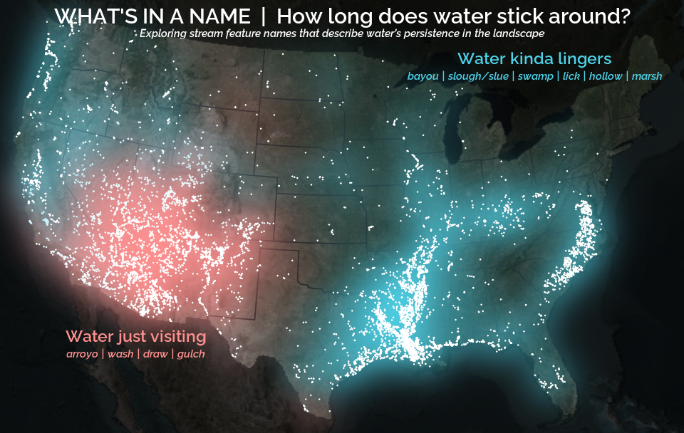
A map that glows with the vocabulary of water
February 27, 2026
English is the official language and authoritative version of all federal information.
A map that glows with the vocabulary of water
What is your first impression of the map above? To me, it is the shimmer. Thousands of points of light, each one a stream or river, illuminating a darkened basemap. Look closely and a pattern emerges: the country’s waterways form a linguistic constellation. These points are classified not from population data or even explicitly by hydrology. They glow strictly according to the vocabulary used to name them and what can be implied about the hydrology of these streams based on their names.
Purrrfect mini-maps - Visualizing water availability across the U.S.
April 20, 2026
The National Water Availability Assessment Data Companion provides nationally-consistent modeled water data, including the surface water supply and use index (SUI) , which is an indication of water limitation across the lower 48 United States. This tutorial shows how to plot monthly SUI from 2010 to 2020 across the lower 48 United States.
Reproducible Data Science in R: Say the quiet part out loud with assertion tests
September 2, 2025

Overview
This blog post is part of the Reprodicuble data science in R series that works up from functional programming foundations through the use of the targets R package to create efficient, reproducible data workflows.
Reproducible Data Science in R: Flexible functions using tidy evaluation
December 17, 2024

Overview
This blog post is part of a series that works up from functional programming foundations through the use of the targets R package to create efficient, reproducible data workflows.
Reproducible Data Science in R: Iterate, don't duplicate
July 18, 2024

Overview
This blog post is part of a series that works up from functional programming foundations through the use of the targets R package to create efficient, reproducible data workflows.