
Large Data Pulls from Water Quality Portal - A Pipeline-Based Approach
A pipeline-based approach for making large data pulls from Water Quality Portal
Background
The Water Quality Portal (WQP
)
database aggregates and standardizes discrete water quality data from
numerous federal, state, tribal, and other monitoring agencies. The WQP
enables the access and retrieval of over 297,000,000 water quality
records (Read et al. 2017) through web services and an application
programming interface (API) that can be called programmatically using
the
dataRetrieval
package in R. Downloading data from the WQP represents a common pattern
across USGS data teams.
In this post, we highlight an example data pipeline to increase the reusability, reproducibility, and efficiency of WQP data workflows. This post is an alternative method to the script-based workflow presented in Large sample pulls using dataRetrieval . We’ve designed it with large-scale data pulls in mind, but this example pipeline will work at any spatial or temporal scale.
Why targets?
The workflow described here uses the targets
package to leverage modular functions, dependency tracking, and automated workflows to inventory and download data from the Water Quality Portal. Using targets allows the user to develop a maintainable pipeline that tracks changes over time and will only re-run portions of the workflow that are out of date due to those changes.
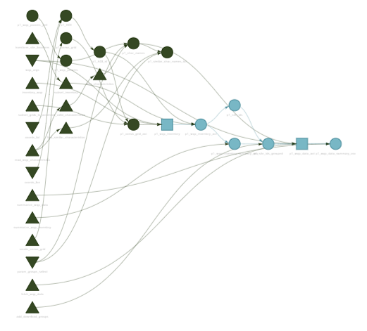
The basic ingredient of a targets workflow is a script file named _targets.R. This file is used to define and configure all of the steps in an analysis pipeline and their connections to each other. After connecting the individual analysis steps (also known as targets) in the _targets file, the targets package can then track the relationships between each connection. Analysis steps that precede any given step of interest are considered “upstream” while the analysis steps that follow are considered “downstream”. Once these connections have been established, targets can also visualize the relationships in a network graph like the one shown below. The WQP pipeline is structured so that various inputs - including the date range, spatial extent, parameters of interest, and/or specific arguments to pass along to WQP queries - can all be modified within the _targets.R
file.
Pulling data from the Water Quality Portal
The WQP targets pipeline is divided into three phases that divide the workflow:
- Inventory what sites and records are available in the WQP
- Download the inventoried data
- Harmonize , or clean, the downloaded data to prepare the dataset for further analysis
This post will focus on how to carry out bulk data pulls using the first two phases of the pipeline.
Decide which characteristic names to query
The first step is to decide which water quality parameters should be
included in the data pull. One challenge posed by the aggregated WQP
database is that many characteristic names may refer to the same water
quality parameter (e.g., temperature records can take on different values
for CharacteristicName, including "Temperature" or
"Temperature, water"). The WQP pipeline includes a configuration file
to help map various WQP characteristics onto more commonly-used
parameter groups (1_inventory/cfg/wqp_codes.yml
).
Here we are interested in compiling temperature data, so we define this
parameter group within _targets.R
.
The characteristic names belonging to “temperature” are parsed in
p1_char_names
to create a vector of CharacteristicName values that
are then used as input to the WQP query. Which values of
CharacteristicName to include may vary depending on the needs of a
specific project and which entries are considered valid in WQP, which can
change over time. To accommodate this variability, the configuration file can be edited to omit
certain characteristic names or include new ones. For example, we might
think of a new characteristic name that contains temperature records and
add that to the configuration file. This simple example illustrates a
decision that users of WQP data must make, but that can sometimes be
difficult to do so with confidence (i.e., is “temp” really a valid
characteristic name?). Two pipeline features are designed to
assist the user when making these decisions. First, all requested
characteristic names from the configuration file are checked against a
list of valid entries in WQP, and will notify the user if a
characteristic name is not valid.
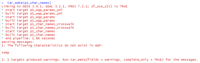
So we can see that our newly-added characteristic name “temp” is not a
valid entry and can be omitted from the configuration file. Second,
a user may wonder whether there are other characteristic names they
might have missed. The pipeline includes a target
p1_similar_char_names_txt
that uses fuzzy string
matching
to
check for valid characteristics that are similar to the requested
parameters, and return an output file that can be evaluated by the user.
In p1_char_names we end up with a list of characteristic names to use
in the query:
> tar_load(p1_char_names)
> p1_char_names
[1] "Temperature"               "Temperature, sample"       "Temperature, water"        "Temperature, water, deg F"
>
Define the area of interest
The next step is to define the spatial extent of the data pull. In this
example, we are requesting data for a triangular “watershed” northwest
of Philadelphia, PA, which we’ve specified in _targets.R
using a set
of latitude and longitude coordinates.
# Specify coordinates that define the spatial area of interest
# lat/lon are referenced to WGS84
coords_lon <- c(-77.063, -75.333, -75.437)
coords_lat <- c(40.547, 41.029, 39.880)
Although we use spatial coordinates, a user could also easily use other,
predefined boundaries by replacing the targets p1_AOI and p1_AOI_sf
with targets that download and read in an external shapefile:
# Download a shapefile containing the Delaware River Basin boundary
  tar_target(
    p1_shp_zip,
    {
      fileout <- "1_inventory/out/drbbnd.zip"
      utils::download.file("https://www.state.nj.us/drbc/library/documents/GIS/drbbnd.zip",
                  destfile = fileout,
                  mode = "wb", quiet = TRUE)
      fileout
    },
    format = "file"
  ),

# Unzip the shapefile and read in as an sf polygon object
  tar_target(
    p1_AOI_sf,
    {
      savedir <- tools::file_path_sans_ext(p1_shp_zip)
      unzip(zipfile = p1_shp_zip, exdir = savedir, overwrite = TRUE)
      sf::st_read(paste0(savedir,"/drb_bnd_arc.shp"), quiet = TRUE) %>%
        sf::st_cast(.,"POLYGON")
    }
  ),
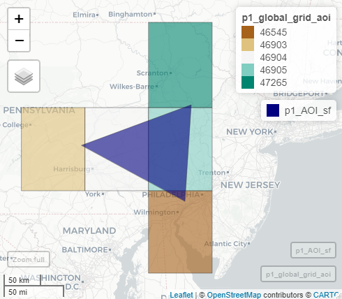
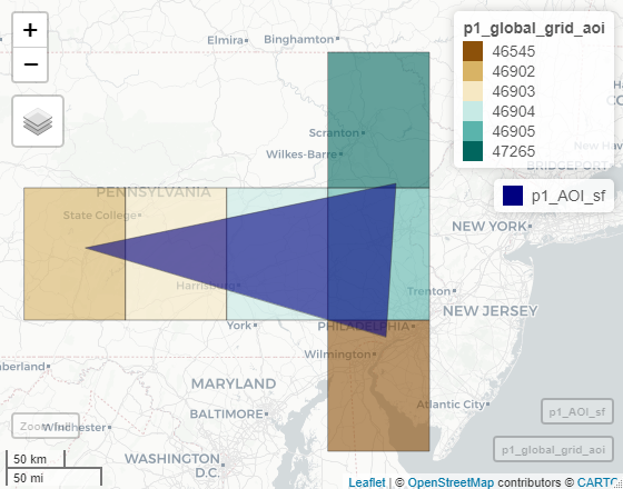
In this example, the area of interest is relatively small and we could probably request all of the temperature data within the boundary of our triangular watershed without issue. However, what if we wanted to download WQP data for the full state of Pennsylvania? This would result in a much bigger request! The WQP pipeline is built around the central idea that smaller queries to the WQP are more likely to succeed and therefore, most workflows that pull WQP data would benefit from dividing larger requests into smaller ones.
One way we break up larger data pulls is by using a set of grid cells to define the spatial extent of multiple, smaller queries that, when combined, represent a data inventory for the full area of interest. The size of each grid cell can be customized by the user, but using 1 degree cell sizes results in a set of five grid cells that overlap our example watershed:
Inventory the data before downloading
We use targets
“branching”
capabilities to apply (or map) our data inventory and download
functions over each grid cell that overlaps our area of interest. The
user can quickly reference the number of sites and records that were
returned in the inventory by referencing a saved log file. If using the
pipeline along with git for version control, this log file also allows
a user to readily track changes to the data over the time.
Little by little: break up the inventoried sites to prepare for download
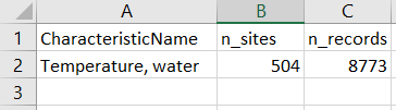
The initial data inventory lets us know how many sites and records we
can expect for each unique CharacteristicName in our query. Before
actually downloading the data, we bin the inventoried sites within each
grid cell into distinct download groups so that the total number of
records in any given download group does not exceed a user-specified maximum
threshold (defaults to 250,000 records per download group
). This binning
step acts as another safeguard against timeout issues with large data
requests, but also allows us to take advantage of targets dependency
tracking to efficiently build or update the data pipeline. For example,
we do not have to re-download all of the data records from WQP just
because we added a new characteristic name or because new sites
were recently uploaded to WQP and detected in our inventory. targets
will only update those data subsets that become “outdated” by an
upstream change.
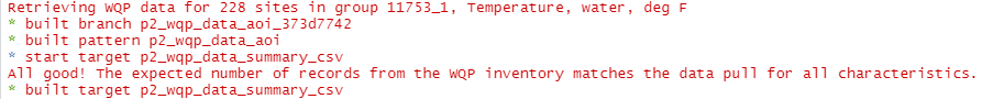
Download the data!
We’re finally ready to download the data from the Water Quality Portal
and do so by mapping the function fetch_wqp_data()
over each unique
download group recombining the data in
p2_wqp_data_aoi. As a check on our downloaded data, we compare the
expected number of sites and records from p1_wqp_inventory_summary_csv
against the number of sites and records that were actually downloaded,
and inform the user of the result:
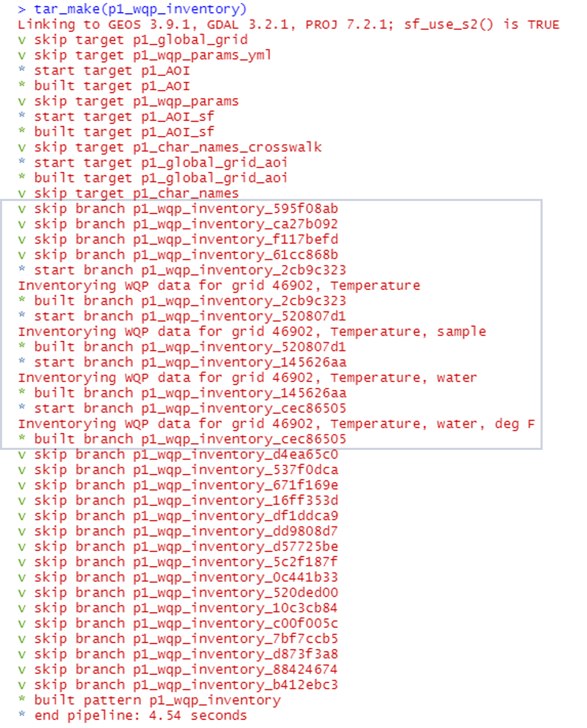
Updating the data pull
As we mentioned above, targets dependency tracking allows us to
efficiently update our pipeline or expand our region of interest without
re-pulling grids that have already been queried. To illustrate, say we
decide to expand an analysis to include areas west of our initial focal
watershed. The map below shows that the area of interest now overlaps six
grid cells instead of five, but the five original grids are still
included in our query. Using common scripting workflows we would usually
just re-pull all of the data again even though that is time-consuming.
However, targets recognizes that data has already been inventoried for
five of these grid cells and will only query data for the newly-added
grid, 46902:
Customizing the pipeline
Our goal is for you to take this example pipeline and tailor it to your own projects. Users can customize the spatial extent, the date range, the list of water quality parameters of interest, and add new functions for harmonizing data for various water quality constituents.
Disclaimer
Any use of trade, firm, or product names is for descriptive purposes only and does not imply endorsement by the U.S. Government.
References
Read, E. K., Carr, L., De Cicco, L., Dugan, H. A., Hanson, P. C., Hart, J. A., Kreft, J., Read, J. S., and Winslow, L. A. (2017), Water quality data for national-scale aquatic research: The Water Quality Portal, Water Resour. Res., 53, 1735– 1745, doi:10.1002/2016WR019993 .
Categories:
Related Posts
Purrrfect mini-maps - Visualizing water availability across the U.S.
April 20, 2026
The National Water Availability Assessment Data Companion provides nationally-consistent modeled water data, including the surface water supply and use index (SUI) , which is an indication of water limitation across the lower 48 United States. This tutorial shows how to plot monthly SUI from 2010 to 2020 across the lower 48 United States.
A map that glows with the vocabulary of water
February 27, 2026
English is the official language and authoritative version of all federal information.
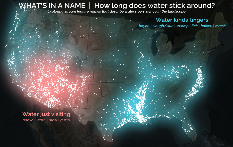
A map that glows with the vocabulary of water
What is your first impression of the map above? To me, it is the shimmer. Thousands of points of light, each one a stream or river, illuminating a darkened basemap. Look closely and a pattern emerges: the country’s waterways form a linguistic constellation. These points are classified not from population data or even explicitly by hydrology. They glow strictly according to the vocabulary used to name them and what can be implied about the hydrology of these streams based on their names.
Extracting the grammar of U.S. stream names
February 27, 2026
English is the official language and authoritative version of all federal information.
Extracting a stream’s feature
The names of streams (hydronyms ) contain, hidden within them, the power to show us the linguistic patterns within the United States. In the United States, stream names tend to follow a binomial structure: a specific name (“Moose,” “Columbia,” “Snake”) paired with a generic feature word (“creek,” “river,” “fork,” “bayou”). The specific portion is endlessly variable, but the generic part is surprisingly stable. In fact, if you look at stream names across the country, the diversity of generic terms is relatively small, but shaped by centuries of hydrologic realities, settlement history, and local tradition.
Reproducible Data Science in R: Say the quiet part out loud with assertion tests
September 2, 2025
Overview
This blog post is part of the Reprodicuble data science in R series that works up from functional programming foundations through the use of the targets R package to create efficient, reproducible data workflows.
Reproducible Data Science in R: Flexible functions using tidy evaluation
December 17, 2024
Overview
This blog post is part of a series that works up from functional programming foundations through the use of the targets R package to create efficient, reproducible data workflows.