Accessing LOCA Downscaling Via OPeNDAP and the Geo Data Portal with R.
Introduction
In this example, we will use the R programming language to access LOCA data via the OPeNDAP web service interface using the ncdf4
package then use the geoknife
package to access LOCA data using the Geo Data Portal
as a geoprocessing service. More examples like this can be found at the Geo Data Portal wiki.
A number of other packages are required for this example. They include: tidyr for preparing data to plot; ggplot2 to create the plots; grid and gridExtra to layout multiple plots in the same figure; jsonlite and leaflet to create the simple map of a polygon; and chron, climates, and PCICt to calculate derived climate indices. They are all available from CRAN
except climates which can be installed from github.
About LOCA
This new, feely available, statistically downscaled dataset is summarized in depth at the U.C. San Diego home web page: Summary of Projections and Additional Documentation
From the Metadata: LOCA is a statistical downscaling technique that uses past history to add improved fine-scale detail to global climate models. We have used LOCA to downscale 32 global climate models from the CMIP5 archive at a 1/16th degree spatial resolution, covering North America from central Mexico through Southern Canada. The historical period is 1950-2005, and there are two future scenarios available: RCP 4.5 and RCP 8.5 over the period 2006-2100 (although some models stop in 2099). The variables currently available are daily minimum and maximum temperature, and daily precipitation. For more information visit: http://loca.ucsd.edu/ The LOCA data is available due to generous support from the following agencies: The California Energy Commission (CEC), USACE Climate Preparedness and Resilience Program and US Bureau of Reclamation, US Department of Interior/USGS via the Southwest Climate Science Center, NOAA RISA program through the California Nevada Applications Program (CNAP), NASA through the NASA Earth Exchange and Advanced Supercomputing (NAS) Division Reference: Pierce, D. W., D. R. Cayan, and B. L. Thrasher, 2014: Statistical downscaling using Localized Constructed Analogs (LOCA). Journal of Hydrometeorology, volume 15, page 2558-2585.
OPeNDAP Web Service Data Access
We’ll use the LOCA Future dataset available from the cida.usgs.gov thredds server.
The OPeNDAP service can be seen here.
and the OPeNDAP base url that we will use with ncdf4 is: http://cida.usgs.gov/thredds/dodsC/loca_future. In the code below, we load the OPeNDAP data source and look at some details about it.
NOTE: The code using ncdf4 below will only work on mac/linux installations of ncdf4. Direct OPeNDAP access to datasets is not supported in the Windows version of ncdf4.
##  [1] "history"              "creation_date"        "Conventions"
##  [4] "title"                "acknowledgment"       "Metadata_Conventions"
##  [7] "summary"              "keywords"             "id"
## [10] "naming_authority"     "cdm_data_type"        "publisher_name"
## [13] "publisher_url"        "creator_name"         "creator_email"
## [16] "time_coverage_start"  "time_coverage_end"    "date_modified"
## [19] "date_issued"          "project"              "publisher_email"
## [22] "geospatial_lat_min"   "geospatial_lat_max"   "geospatial_lon_min"
## [25] "geospatial_lon_max"   "license"
##  [1] "filename"    "writable"    "id"          "safemode"    "format"
##  [6] "is_GMT"      "groups"      "fqgn2Rindex" "ndims"       "natts"
## [11] "dim"         "unlimdimid"  "nvars"       "var"
## [1] "bnds" "lat" "lon" "time"
## [1] 171
From this, we can see the global variables that are available for the dataset as well as the ncdf4 object’s basic structure. Notice that the dataset has 171 variables!
Point-based time series data
For this example, we’ll look at the dataset in the Colorado Platte Drainage Basin climate division which includes Denver and North Central Colorado. For the examples that use a point, well use 40.2 degrees north latitude and 105 degrees west longitude, along I25 between Denver and Fort Collins.
Get time series data for a single cell.
First, let’s pull down a time series from our point of interest using ncdf4. To do this, we need to determine which lat/lon index we are interested in then access a variable of data at that index position.
## [1] "lat 40.21875 lon 254.96875"
## [1] "lat_bnds"                  "lon_bnds"
## [3] "time_bnds"                 "pr_CCSM4_r6i1p1_rcp45"
## [5] "tasmax_CCSM4_r6i1p1_rcp45" "tasmin_CCSM4_r6i1p1_rcp45"
## [7] "pr_CCSM4_r6i1p1_rcp85"     "tasmax_CCSM4_r6i1p1_rcp85"
## [9] "tasmin_CCSM4_r6i1p1_rcp85"
## Time difference of 1.653601 mins
Time series plot of two scenarios.
In the code above, we requested the fifth variable, or tasmax_CCSM4_r6i1p1_rcp45. Let’s request a second variable and see how rcp45 compares to rcp85. For this example, we’ll need three additional packages: chron to deal with the NetCDF time index conversion, tidyr to get data ready to plot with the gather function, and ggplot2 to create a plot of the data.
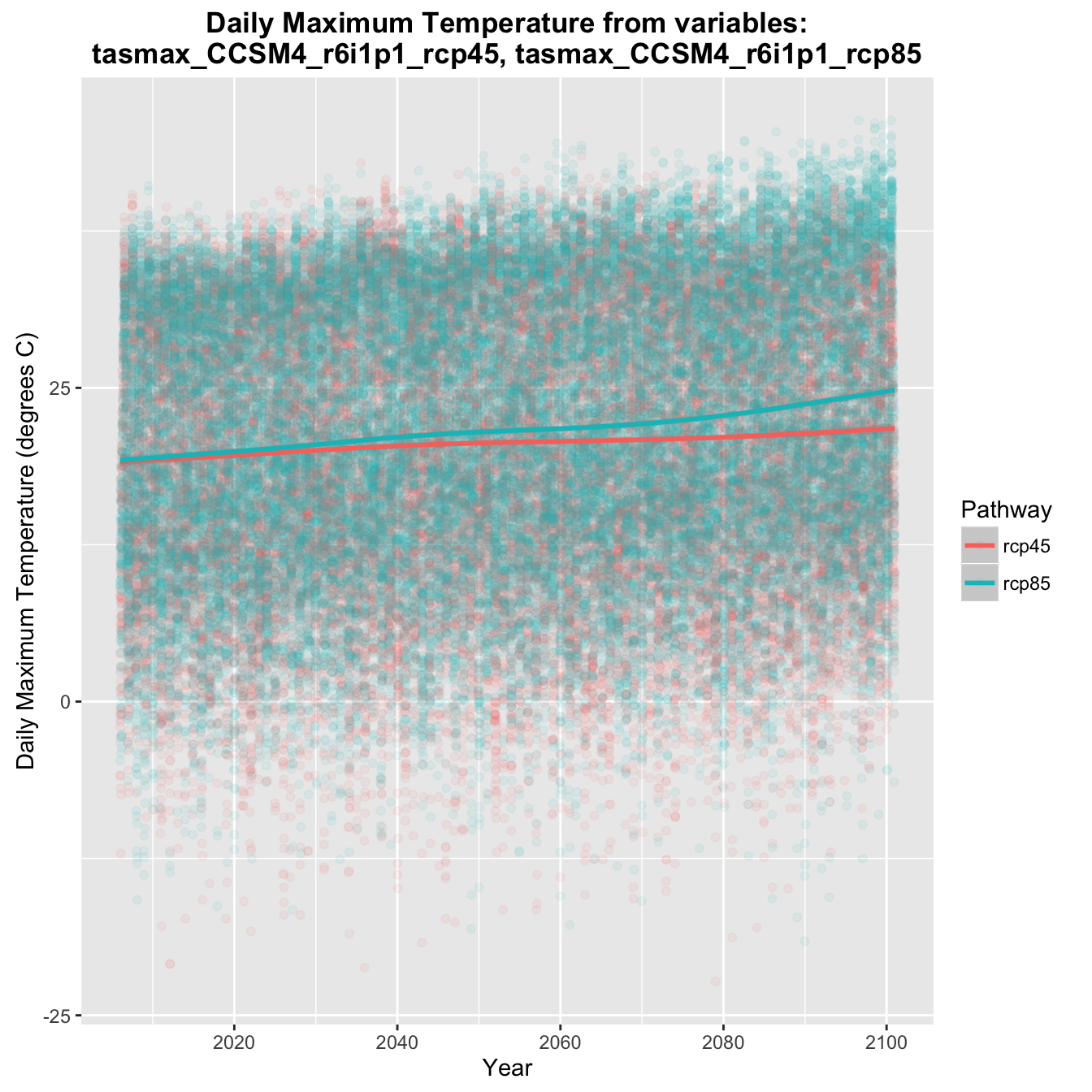
Graph of projected daily maximum temperature.
Areal average time series data access with the Geo Data Portal
Using the method shown above, you can access any variable at any lat/lon location for your application. Next, we’ll look at how to get areal statistics of the data for the Platte Drainage Basin climate division polygon shown above.
For this, we’ll need the package geoknife. In the code below, we setup the webgeom and webdata objects called stencil and fabric respectively. Then we make a request for one timestep to find out the SUM of the cell weights and the total COUNT of cells in the area weighted grid statistics calculation that the Geo Data Portal will perform at the request of geoknife. This tells us the fractional number of grid cells considered in the calculation as well as the total number of cells that will be considered for each time step.
##              DateTime PLATTE DRAINAGE BASIN              variable
## 1 2006-01-01 12:00:00              1465.039 pr_CCSM4_r6i1p1_rcp45
## 2 2006-01-01 12:00:00              1616.000 pr_CCSM4_r6i1p1_rcp45
##   statistic
## 1       SUM
## 2     COUNT
Areal intersection calculation summary
This result shows that the SUM and COUNT are 1465.039 and 1616 respectively. This tells us that of the 1616 grid cells that partially overalap the Platte Drainage Basin polygon, the sum of cell weights in the area weighted grid statistics calculation is 1465.039. The Platte Drainage Basin climate division is about 52,200 square kilometers and the LOCA grid cells are roughly 36 square kilometers (1/16th degree). Given this, we would expect about 1450 grid cells in the Platte Drainage Basin polygon which compares will with the Geo Data Portal’s 1465.
Process time and request size analysis
Next, we’ll look at the time it might take to process this data with the Geo Data Portal. We’ll use the geoknife setup from above, but the default knife settings rather than those used above to get the SUM and COUNT. First we’ll get a single time step, then a year of data. Then we can figure out how long the spatial interstection step as well as each time step should take.
## Precip time is about 0.4170167 hours per variable.
## Time for spatial intersection is about 6.68374 seconds.
This result shows about how long we can expect each full variable to take to process and how much of that process is made up by the spatial intersection calculations. As can be seen, the spatial intersection is insignificant compared to the time series data processing, which means running one variable at a time should be ok.
In the case that the spatial intersection takes a lot of time and the data processing is quick, we could run many variables at a time to limit the number of spatial intersections that are performed. In this case, we can just run a single variable per request to geoknife and the Geo Data Portal.
GDP run to get all the data.
Now, lets run the GDP for the whole loca dataset. This will be 168 variables with each variable taking something like a half hour depending on server load. Assuming 30 minutes per variable, that is 84 hours! That may seem like a very long time, but considering that each variable is 34310 time steps, that is a throughput of about 19 time steps per second.
The code below is designed to keep retrying until the processing result for each has been downloaded successfully. For this demonstration, the processing has been completed and all the files are available in the working directory of the script. NOTE: This is designed to make one request at a time. Please don’t make concurrent requests to the GDP, it tends to be slower than executing them in serial.
Derivative calculations
Now that we have all the data downloaded and it has been parsed into a list we can work with, we can do something interesting with it. The code below shows an example that uses the climates package, available on github
to generate some annual indices of the daily data we accessed. For this example, we’ll look at all the data and 5 derived quantities.
Plot setup
Now we have a data in a structure that we can use to create some plots. First, we define a function from the ggplot2 wiki that allows multiple plots to share a legend.
Summary Plots
Now we can create a set of plot configuration options and a set of comparitive plots looking at the RCP45 (aggressive emmisions reduction) and RCP85 (business as usual).
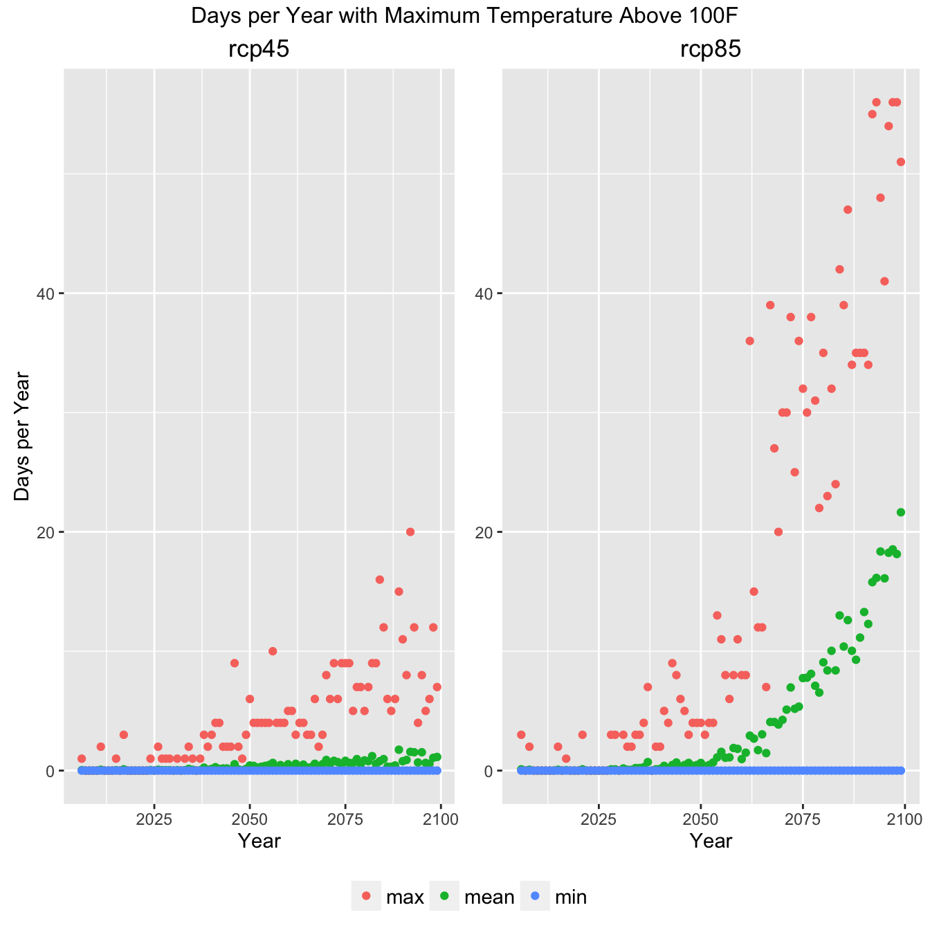
Climate Indicator Summary Graph
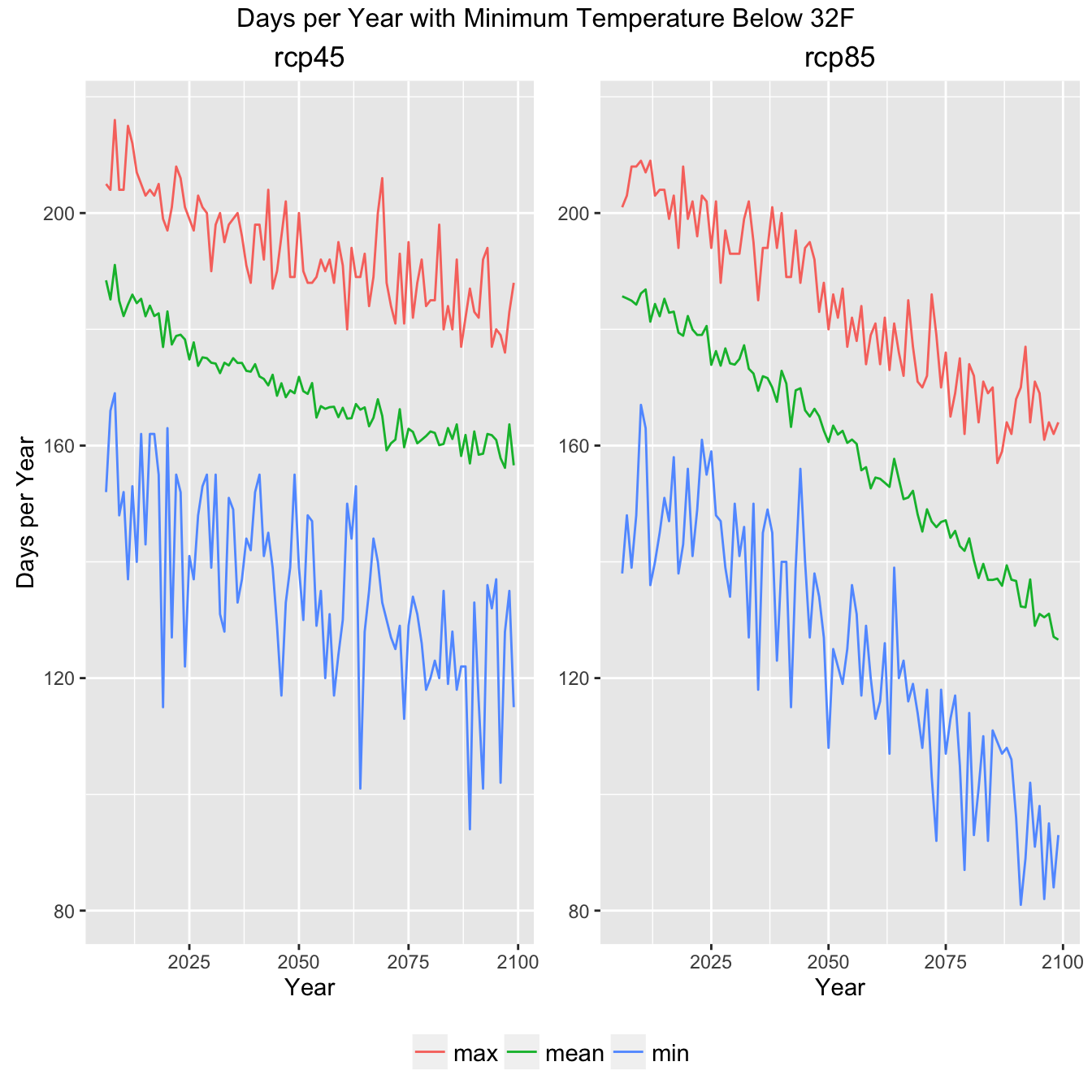
Climate Indicator Summary Graph
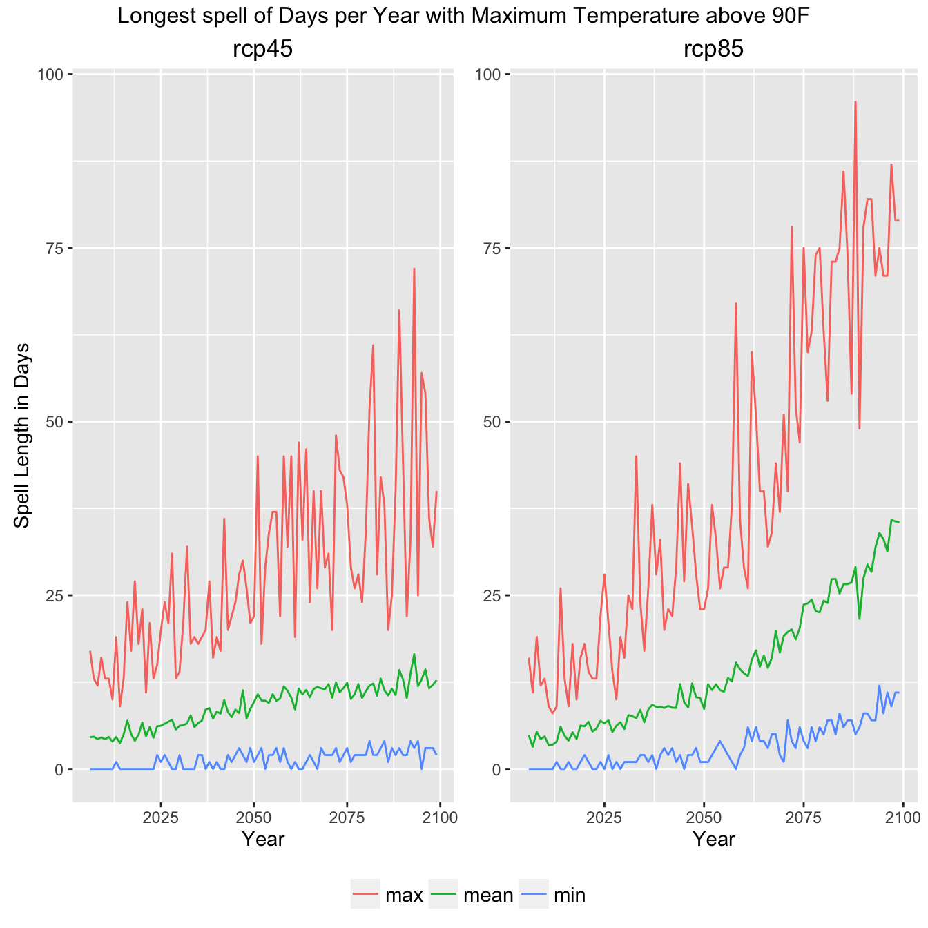
Climate Indicator Summary Graph
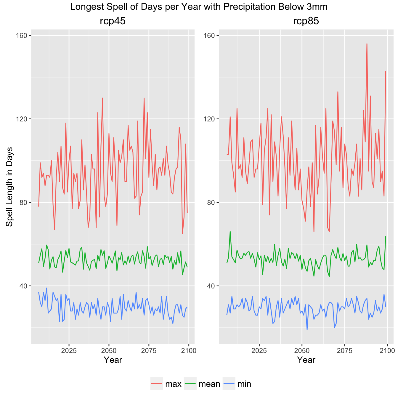
Climate Indicator Summary Graph
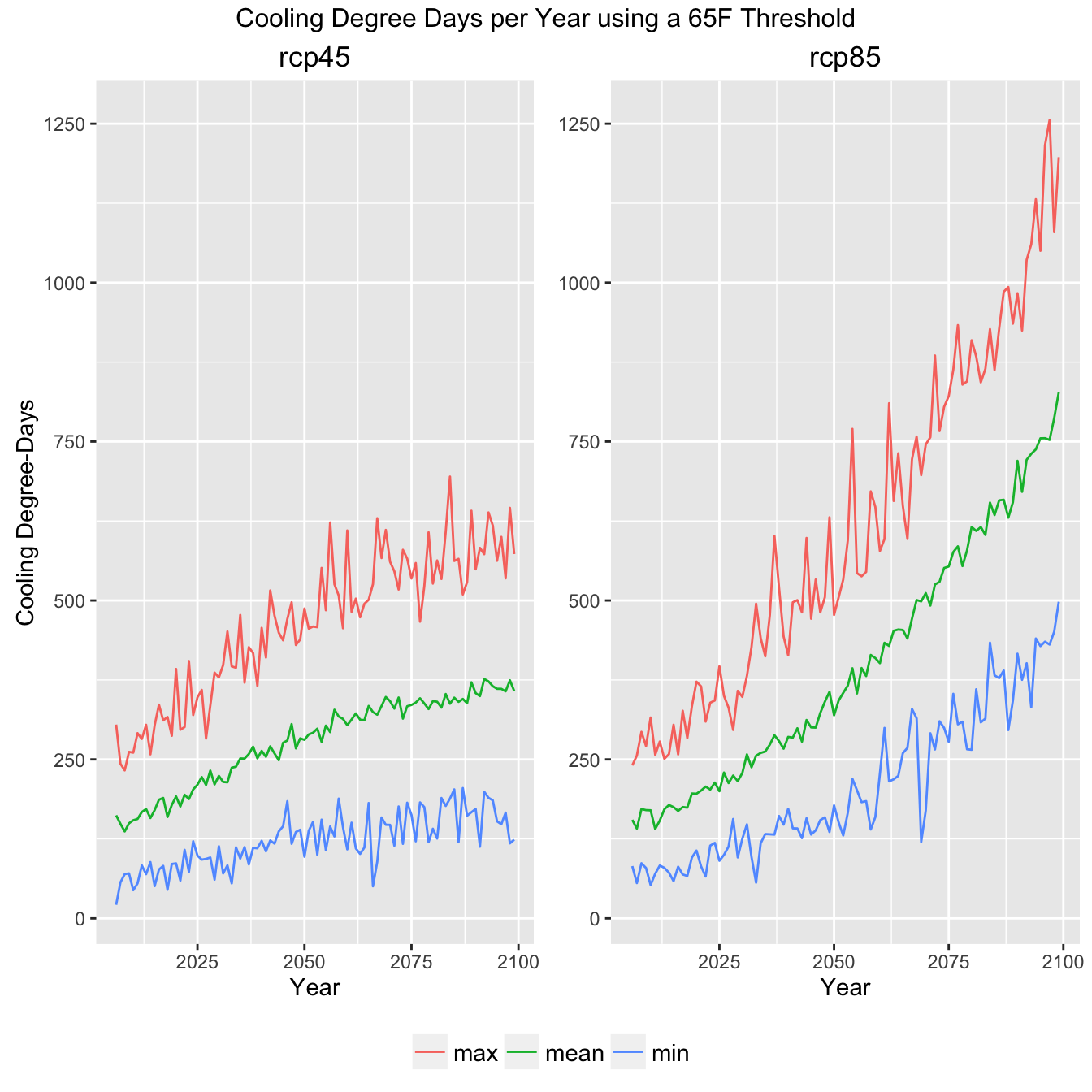
Climate Indicator Summary Graph
All GCM Plots
Finally, to give an impression of how much data this example actually pulled in, here are the same plots with all the GCMs shown rather then the ensemble mean, min, and max.
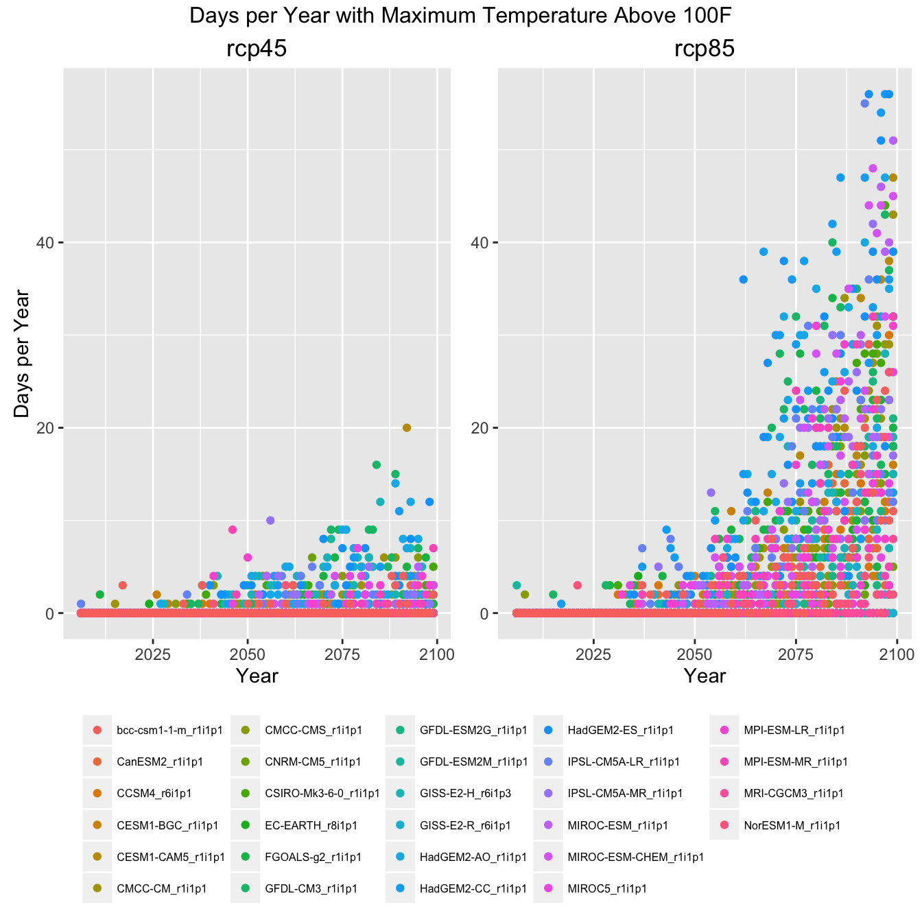
Climate Indicator Graph of All GCMs
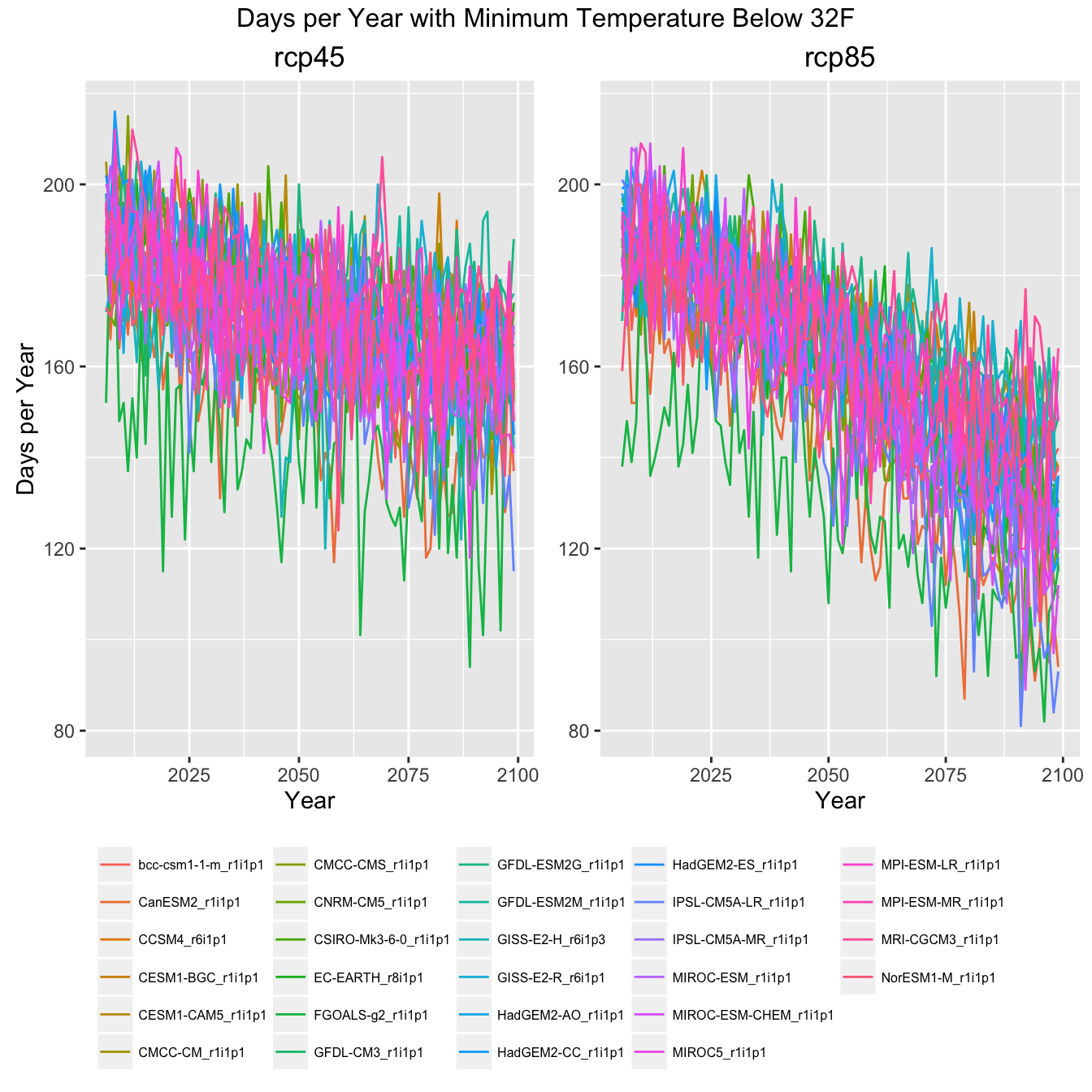
Climate Indicator Graph of All GCMs
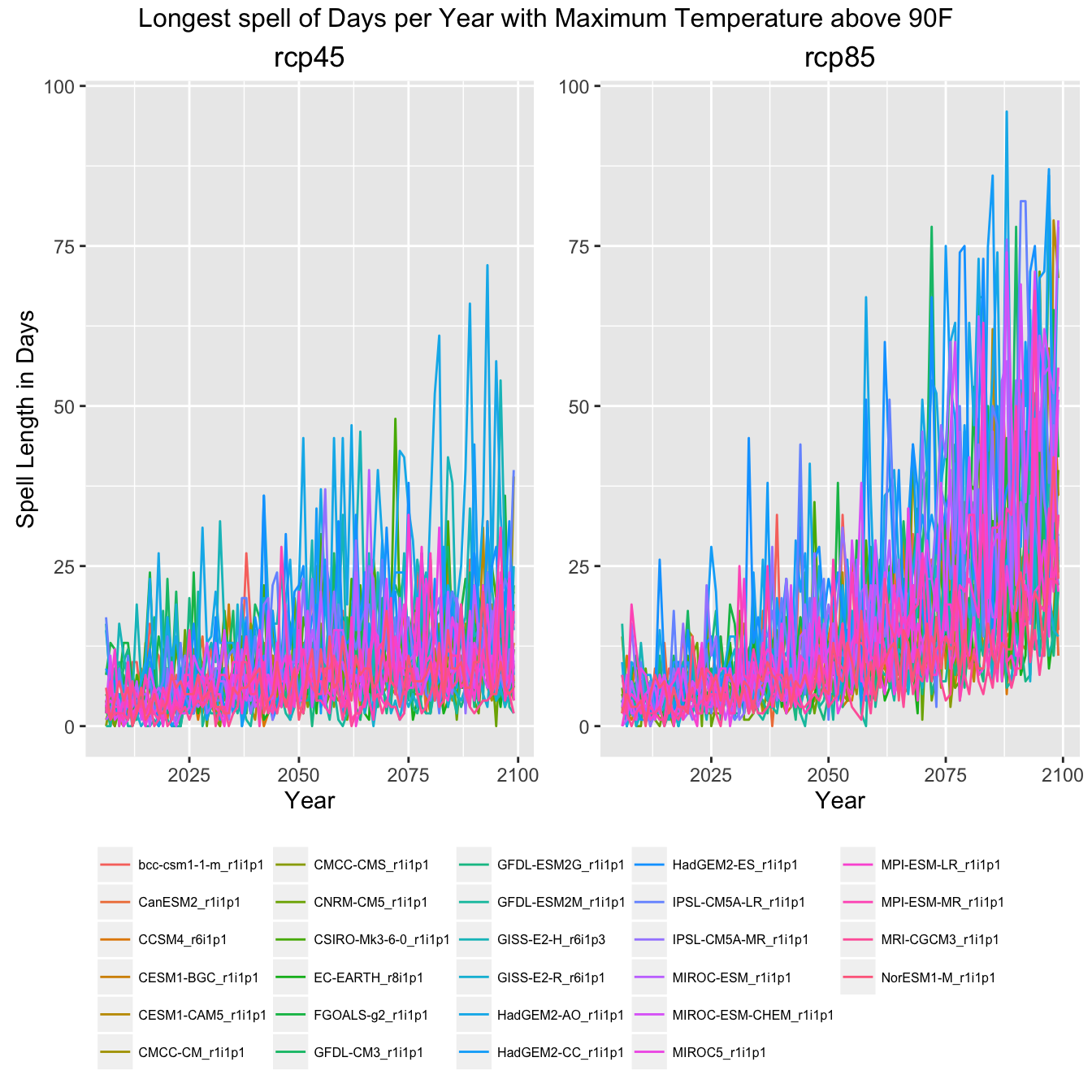
Climate Indicator Graph of All GCMs
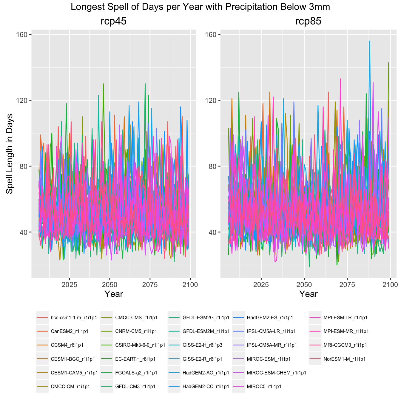
Climate Indicator Graph of All GCMs
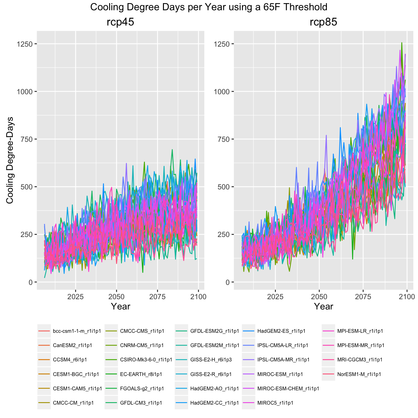
Climate Indicator Graph of All GCMs
Categories:
Related Posts
Visualizing Tropical Storm Colin Precipitation using geoknife
June 9, 2016
Tropical Storm Colin (TS Colin) made landfall on June 6 in western Florida. The storm moved up the east coast, hitting Georgia, South Carolina, and North Carolina.
The Hydro Network-Linked Data Index
November 2, 2020
Introduction updated 11-2-2020 after updates described here . updated 9-20-2024 when the NLDI moved from labs.waterdata.usgs.gov to api.water.usgs.gov/nldi/ The Hydro Network-Linked Data Index (NLDI) is a system that can index data to NHDPlus V2 catchments and offers a search service to discover indexed information.
Seasonal Analysis in EGRET
November 29, 2016
Introduction This document describes how to obtain seasonal information from the R package EGRET . For example, we might want to know the fraction of the load that takes place in the winter season (say that is December, January, and February).
Calculating Moving Averages and Historical Flow Quantiles
October 25, 2016
This post will show simple way to calculate moving averages, calculate historical-flow quantiles, and plot that information. The goal is to reproduce the graph at this link: PA Graph .
The case for reproducibility
October 6, 2016
Science is hard. Why make it harder? Scientists and researchers spend a lot of time on data preparation and analysis, and some of these analyses are quite computationally intensive.

