Tutorial of dataRetrieval's newest features in R

This is a basic dataRetrieval tutorial for USGS water data in R in which we highlight new functionality for dataRetrieval and the new Water Data APIs.

This article will describe the R-package dataRetrieval , which simplifies the process of finding and retrieving water from the U.S. Geological Survey (USGS) and other agencies. We have recently released a new version of dataRetrieval to work with the modernized Water Data APIs . The new version of dataRetrieval has several benefits for new and existing users:

1. Human-readable function names and arguments written in “snake case” (e.g., read_waterdata_samples())
2. Customized functions for each of the Water Data API services (e.g., latest continuous values) plus a generic function that covers all services
3. API token registration option to overcome new limits on how many queries can be requested per IP address per hour. Visit https://api.waterdata.usgs.gov/signup/ for a token.
4. The new functions include ALL possible arguments that the web service APIs support
5. And, as always, continued development of dataRetrieval versions and documentation

This blog is not an exhaustive guide to all of the new functions, arguments, and capabilities of dataRetrieval. Instead, it demonstrates some common use cases for retrieving USGS water data information in R while highlighting how the new features work differently (and we would argue better) than the old features.

Globally defined output fields now also function as arguments

This is one of the more flexible and user-friendly features of the new dataRetrieval package. For all new retrieval functions, there are a set series of possible arguments that can be used to retrieve data. For example, with the dataRetrieval::read_waterdata_monitoring_location() function, input arguments can include:

• monitoring_location_id such as "USGS-01491000", which would retrieve just this one unique monitoring location
• hydrologic_unit_code such as "010600050203", which would retrieve all monitoring locations in this 12-unit hydrologic area
• state_name such as "Maryland", which would retrieve all monitoring locations in this state

The cool thing now is that those are also fields that are returned: the input arguments and the returning field names are the same! You can use the properties argument in your retrieval function to return only the properties you want. To view a list of the arguments for a given function, view the Function Help page of the dataRetrieval site.The next two examples show you how to interchange between arguments for retrieval and the properties you retrieve.

Example: Retrieve one specific monitoring location

In this example, we will specifically look for one monitoring location based on the monitoring_location_id. Often (but not always), these IDs are 8 digits for surface-water sites and 15 digits for groundwater sites. The first step to finding data is discovering the monitoring_location_id. A great place to start looking is on the National Water Dashboard .

About Monitoring Location Data: The USGS organizes hydrologic data in a standard structure. Monitoring locations are located throughout the United States, and each location has a unique ID (referred in this document and throughout the dataRetrieval package in one of three formats:

• monitoring_location_number: Each monitoring location in the USGS data base has a unique 8- to 15-digit identification number. Monitoring location numbers are assigned based on this logic.
• monitoring_location_id: Monitoring location IDs are created by combining the agency code of the agency responsible for the monitoring location (e.g. “USGS”) with the ID number of the monitoring location (e.g. “02238500”), separated by a hyphen (e.g. “USGS-02238500 ”).
• monitoring_location_name: This is the official name of the monitoring location in the database. For well information this can be a district-assigned local number.

As we download the data, we will specify that we only want to return the monitoring_location_id, state_name and hydrologic_unit_code. Note that a geometry field is returned alongside the selected “properties” (more on this in a minute).

out_sf <- 
  dataRetrieval::read_waterdata_monitoring_location(
    monitoring_location_id = "USGS-01491000", 
    properties = c("monitoring_location_id", "state_name", "hydrologic_unit_code"))


#> Requesting:
#> https://api.waterdata.usgs.gov/...
#> out_sf
#> Simple feature collection with 1 feature and 3 fields
#> Geometry type: POINT
#> Dimension:     XY
#> Bounding box:  xmin: -75.78581 ymin: 38.99719 xmax: -75.78581 ymax: 38.99719
#> Geodetic CRS:  WGS 84
#> # A tibble: 1 × 4
#>   monitoring_location_id state_name hydrologic_unit_code             geometry
#>   <chr>                  <chr>      <chr>                         <POINT [°]>
#> 1 USGS-01491000          Maryland   020600050203         (-75.78581 38.99719)

Example: Retrieve monitoring locations within a state

In this example, we retrieval all monitoring locations within a state, and also return only the monitoring_location_id, state_name and hydrologic_unit_code fields. Note, monitoring locations can include streamgages, groundwater wells, etc.

out_sf <- 
  dataRetrieval::read_waterdata_monitoring_location(
    state_name = "Maryland", 
    properties = c("monitoring_location_id", "state_name", "hydrologic_unit_code"))


#> Requesting:
#> https://api.waterdata.usgs.gov/...
#>
#> head(out_sf)
#> Simple feature collection with 6 features and 3 fields
#> Geometry type: POINT
#> Dimension:     XY
#> Bounding box:  xmin: -77.63472 ymin: 39.58083 xmax: -77.62582 ymax: 39.59732
#> Geodetic CRS:  WGS 84
#> # A tibble: 6 × 4
#>   monitoring_location_id state_name hydrologic_unit_code             geometry
#>   <chr>                  <chr>      <chr>                         <POINT [°]>
#> 1 MD006-393451077375601  Maryland   020700041007         (-77.63222 39.58083)
#> 2 MD006-393451077380001  Maryland   020700041007         (-77.63333 39.58083)
#> 3 MD006-393452077380501  Maryland   020700041007         (-77.63472 39.58111)
#> 4 MD006-393547077373701  Maryland   020700041007         (-77.62666 39.59649)
#> 5 MD006-393548077373401  Maryland   020700041007         (-77.62582 39.59676)
#> 6 MD006-393550077373701  Maryland   020700041007         (-77.62666 39.59732)

Returning simple features by default

If you’ve been following along, you may have realized that the output from the previous two examples were in the simple features format. This allows for easy interactions with sf package for simple feature manipulation and ggplot2 for simple feature plotting/mapping. The returned data includes a column geometry which is a collection of the simple feature points.

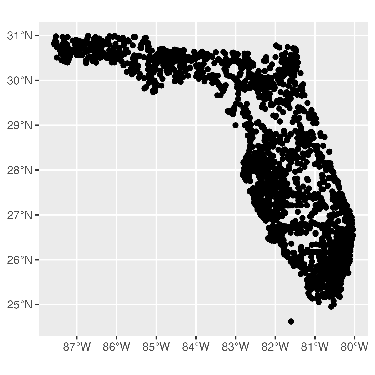
Example: Easily map features directly from dataRetrieval

Let's plot USGS streamgage monitoring locations in Florida. To do this, we'll specify that we want streamgages with the site_type argument, and then filter to USGS sites with the returned agency_code property.

library(ggplot2)

out_sf <- 
  dataRetrieval::read_waterdata_monitoring_location(
    state_name = "Florida", 
    site_type = "Stream",
    properties = c("monitoring_location_id", "agency_code"))

ggplot(data = out_sf) +
  geom_sf()

Returning “long” format data by default

For this example, we’ll retrieve Daily Values from the API service. This new function, read_waterdata_daily() replaces readNWISdv(). The returned simple feature data frame is in a “long” format, which means there is just a single observations per row of the data frame. Many functions will be easier and more efficient to work with in a “long” data frame.

About Daily Values : Daily data provide one data value to represent water conditions for the day. Throughout much of the history of the USGS, the primary water data available was daily data collected manually at the monitoring location once each day. With improved availability of computer storage and automated transmission of data, the daily data published today are generally a statistical summary or metric of the continuous data collected each day, such as the daily mean, minimum, or maximum value. Daily data are automatically calculated from the continuous data of the same parameter code and are described by parameter code and a statistic code.

daily_modern <- dataRetrieval::read_waterdata_daily(
  monitoring_location_id = "USGS-01491000",
  parameter_code = c("00060", "00010"),
  statistic_id = "00003",
  time = c("2023-10-01", "2025-09-15"),
  properties = c("monitoring_location_id", "parameter_code", "time", 
                 "value", "approval_status"))

#> head(daily_modern)
#> Simple feature collection with 6 features and 4 fields
#> Geometry type: POINT
#> Dimension:     XY
#> Bounding box:  xmin: -75.78581 ymin: 38.99719 xmax: -75.78581 ymax: 38.99719
#> Geodetic CRS:  WGS 84
#> # A tibble: 6 × 5
#>  monitoring_location_id parameter_code time       value             geometry
#>   <chr>                  <chr>          <date>     <dbl>          <POINT [°]>
#> 1 USGS-01491000          00010          2023-10-01  18.3 (-75.78581 38.99719)
#> 2 USGS-01491000          00060          2023-10-01  61.9 (-75.78581 38.99719)
#> 3 USGS-01491000          00060          2023-10-02  57.2 (-75.78581 38.99719)
#> 4 USGS-01491000          00010          2023-10-02  19   (-75.78581 38.99719)
#> 5 USGS-01491000          00010          2023-10-03  19.6 (-75.78581 38.99719)
#> 6 USGS-01491000          00060          2023-10-03  44.6 (-75.78581 38.99719)

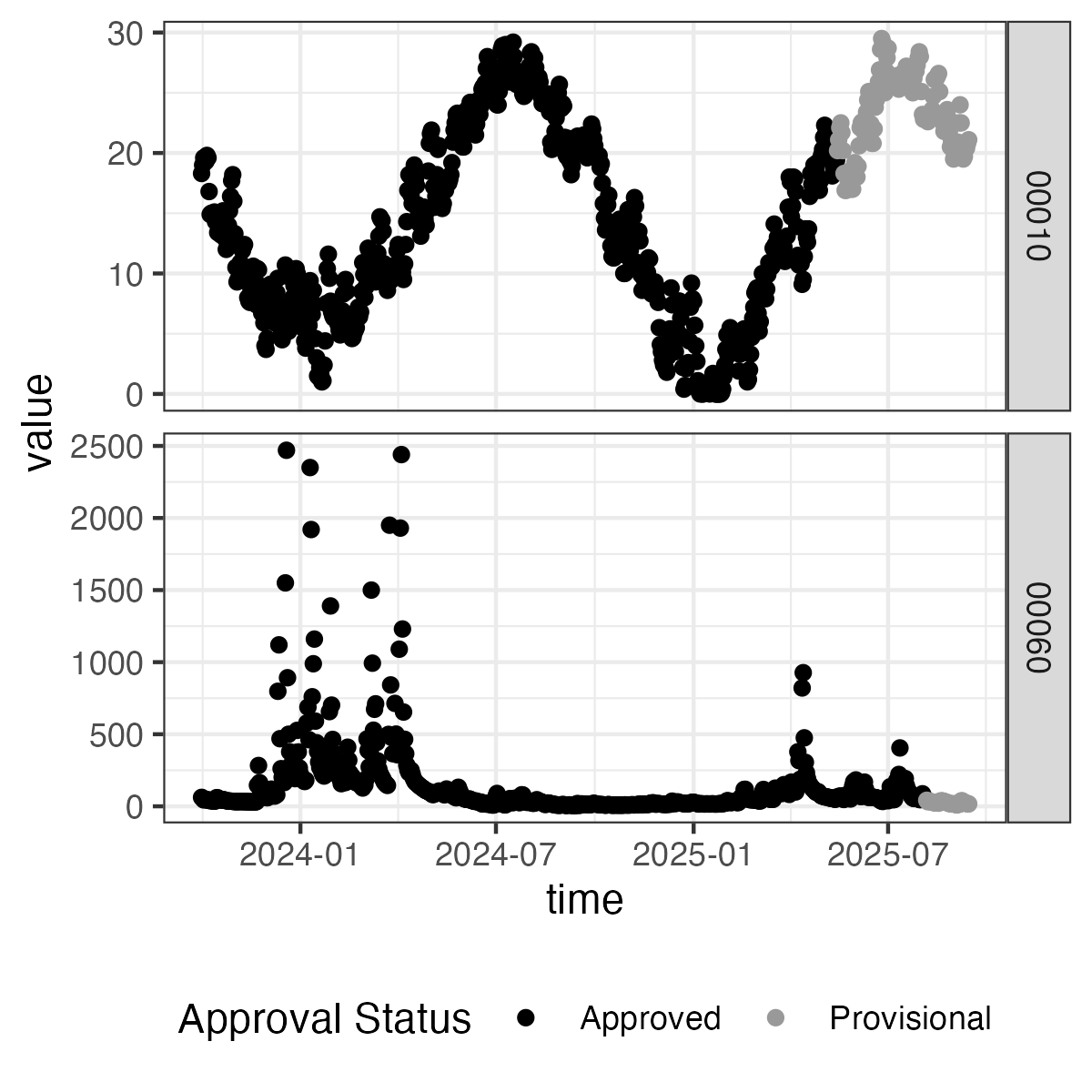
Example: Create a facet plot directly from dataRetrieval

Here we can see how we can use the parameter_code column to create a “facet” plot. We also use the approval_status field mapped to color to show that the provisional data have come out more recently and are not yet in "approved" status.

library(ggplot2)

ggplot(data = daily_modern) +
  geom_point(aes(x = time, y = value, 
                 color = approval_status)) +
  facet_grid(parameter_code ~ ., scale = "free") +
  scale_color_manual(values = c("black", "grey60")) +
  theme_bw() +
  theme(legend.position = "bottom")
  

New capability: Metadata retrieval

These functions are designed to get metadata from Water Data API services . These are useful to get function arguments and other metadata associated with USGS codes.

• read_waterdata_metadata() gives access to a wide variety of tables that have metadata information (e.g., parameter codes or statistics codes )
• read_waterdata_ts_meta() provides metadata about time series, including their operational thresholds, units of measurement, and when the earliest and most recent observations in a time series occurred. Daily data and continuous measurements are queried together with this function; therefore there may be duplicate rows for a given monitoring location. The field computation_period_identifier differentiates these duplicate rows (e.g., a row each for Daily Values, Point Data, and Continuous Data)*

Example: Retrieve aquifer metadata with read_waterdata_metadata()

About groundwater data: Groundwater occurs in aquifers under two different conditions. Where water only partly fills an aquifer, the upper surface is free to rise and decline. These aquifers are referred to as unconfined (or water-table) aquifers. Where water completely fills an aquifer that is overlain by a confining bed, the aquifer is referred to as a confined (or artesian) aquifer. When a confined aquifer is penetrated by a well, the water level in the well will rise above the top of the aquifer (but not necessarily above land surface).

> dataRetrieval::read_waterdata_metadata(collection = "aquifer-types")
#> Requesting:
#> https://api.waterdata.usgs.gov/...
#> # A tibble: 5 × 2
#>   aquifer_type aquifer_type_description                         
#>   <chr>        <chr>                                            
#> 1 C            Confined single aquifer                          
#> 2 M            Confined multiple aquifers                       
#> 3 N            Unconfined multiple aquifer                      
#> 4 U            Unconfined single aquifer                        
#> 5 X            Mixed (confined and unconfined) multiple aquifers
 

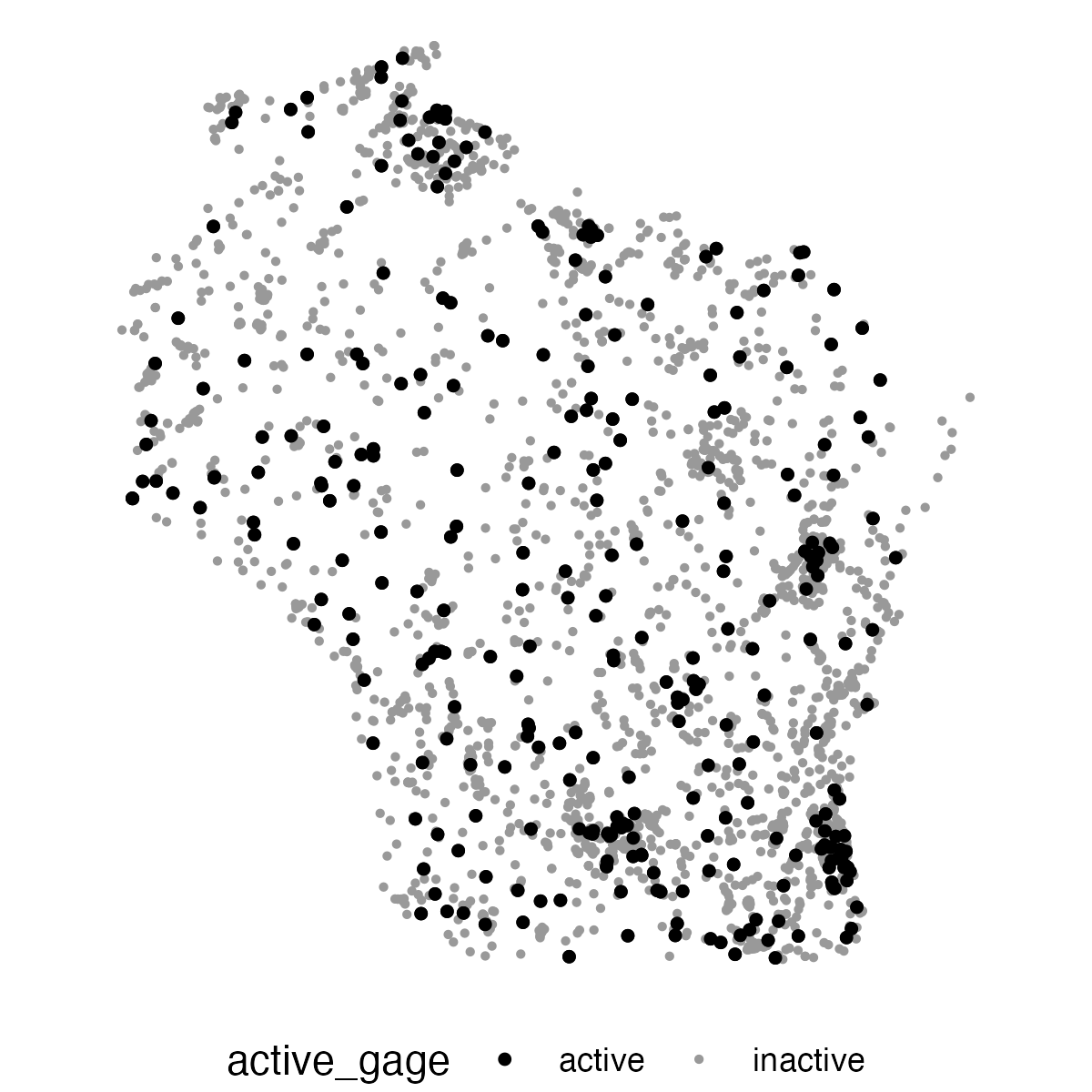
Example: Retrieve and plot active streamgage sites in Wisconsin

Using the read_waterdata_ts_meta() and the argument last_modified, we are able to determine which sites are considered "active." There is a multitude of ways to define an active site, so for the sake of this example we will define active sites as: Monitoring locations that have had data collected from them within the past 13 months.

In this example, we're going to first query for all active sites using our last_modified query. Then, we'll match those to all streamgage sites in Wisconsin and plot the active gages and inactive gages as different colors.

library(dplyr)
library(ggplot2)

# Note, this downloads all records that fit the query, 
#  meaning that there are duplicate monitoring location ids in this sf
active_sites <- dataRetrieval::read_waterdata_ts_meta(
  last_modified = "P13M",
  parameter_name = "Discharge",
  properties = c("monitoring_location_id", "computation_period_identifier")
) 
active_list <- unique(active_sites$monitoring_location_id)

# Download all Wisconsin streamgage monitoring locations
wi_gages <- dataRetrieval::read_waterdata_monitoring_location(
  state_name = "Wisconsin", 
  site_type = "Stream",
  properties = c("monitoring_location_id"))

# Create new field in wi_gages for active in past 13 months
wi_gages <- wi_gages |>
  dplyr::mutate(active_gage = 
    case_when(monitoring_location_id %in% active_list ~ "active",
    TRUE ~ "inactive"))
    
# plot
ggplot(data = wi_gages) +
  geom_sf(aes(color = active_gage, size = active_gage)) +
  # print active sites on top
  geom_sf(data = wi_gages |> dplyr::filter(active_gage == "active"),
    color = "black", size = 1) +
  scale_color_manual(values = c("black", "grey60")) +
  scale_size_manual(values = c(1, 0.5)) +
  theme_void() + 
  theme(legend.position = "bottom")

New function: read_waterdata_latest_continuous()

The read_waterdata_latest_continuous() function does not have an equivalent NWIS function to replace. It is used to get the latest continuous measurement and can be queried using the same arguments as previously demonstrated (e.g., monitoring_location_id)

About latest continuous values: This endpoint provides the most recent observation for each time series of continuous data. Continuous data are collected via automated sensors installed at a monitoring location. They are collected at a high frequency and often at a fixed 15-minute interval. Depending on the specific monitoring location, the data may be transmitted automatically via telemetry and be available on WDFN within minutes of collection, while other times the delivery of data may be delayed if the monitoring location does not have the capacity to automatically transmit data. Continuous data are described by parameter name and parameter code. These data might also be referred to as “instantaneous values” or “IV”

New general retrieval function: read_waterdata()

The read_waterdata() function replaces the readNWISdata function. This is a lower-level, generalized function for querying any of the API endpoints.

The new APIs can handle complex requests. For those queries, users will need to construct their own request using Contextual Query Language (CQL2). There’s an excellent article on CQL2 on the Water Data API webpage .

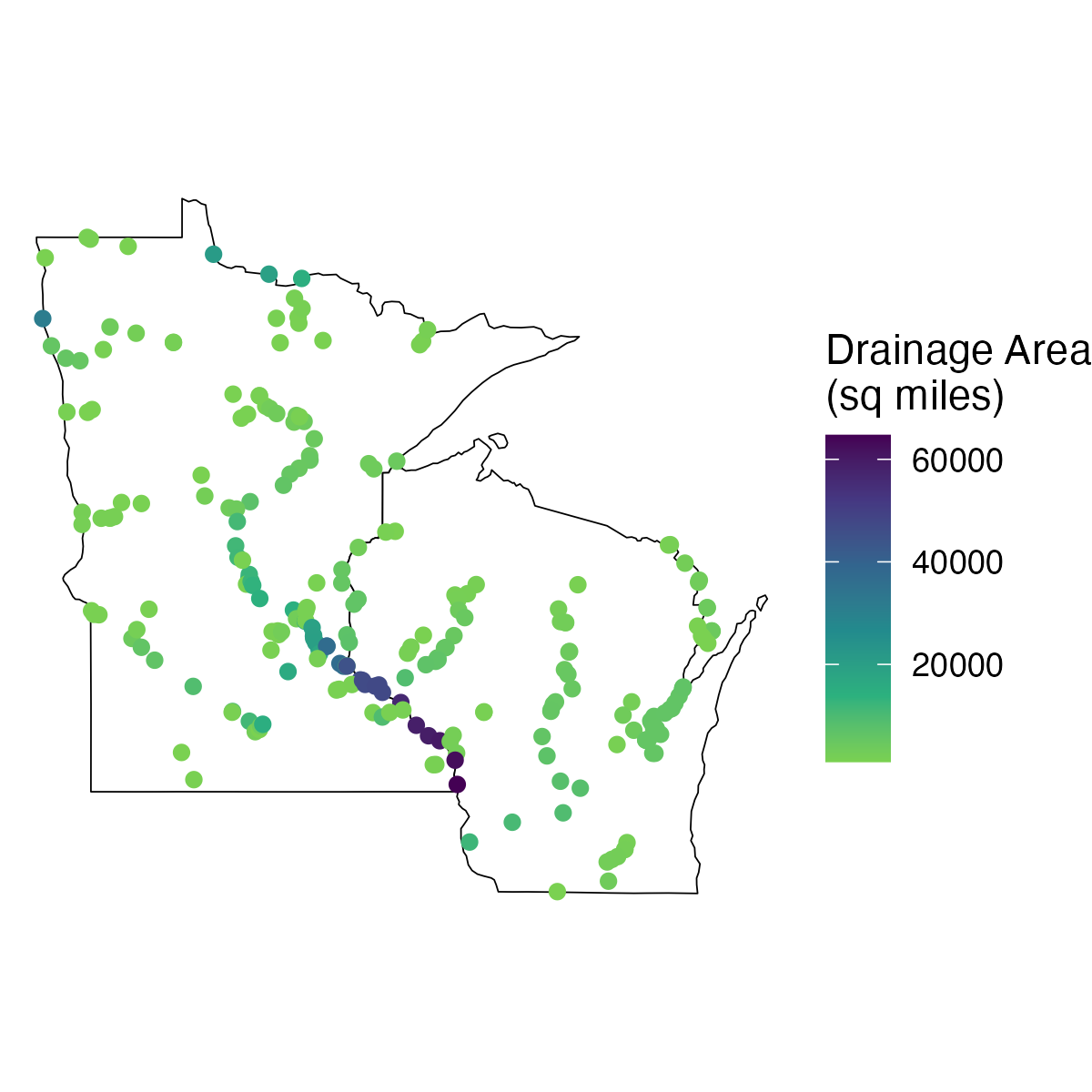
Example: Retrieve data with general retrieval function

Let's find sites in Wisconsin and Minnesota that have a drainage area greater than 1,000 square miles. We'll also map those locations on state outlines using the packages ggplot2 and usmapdata.

cql <- '{
  "op": "and",
  "args": [
    {
      "op": "in",
        "args": [
          { "property": "state_name" },
          [ "Wisconsin", "Minnesota" ]
        ]
    },
    {
      "op": ">",
        "args": [
          { "property": "drainage_area" },
          1000
        ]
    }
  ]
}'

sites_mn_wi <- dataRetrieval::read_waterdata( 
  service = "monitoring-locations", 
  CQL = cql)
  
library(ggplot2)
library(usmapdata)

# Fetch states for map
states <- usmapdata::us_map(regions = "states", 
            include = c("Minnesota", "Wisconsin"))
ggplot(data = sites_mn_wi) +
  geom_sf(data = states, fill = "white", color = "black") +
  geom_sf(aes(color = drainage_area)) +
  scale_color_viridis_c(direction = -1, end = 0.8, name = "Drainage Area\n(sq miles)") +
  theme_void()

Questions?

Questions on dataRetrieval? Create an issue here: https://github.com/DOI-USGS/dataRetrieval/issues

Disclaimer

Any use of trade, firm, or product names is for descriptive purposes only and does not imply endorsement by the U.S. Government.