
Reproducible Data Science in R: Iterate, don't duplicate
Iterate your R code using the map() function from the purrr package.
What's on this page

Overview
This blog post is part of a series that works up from functional programming foundations through the use of the targets R package to create efficient, reproducible data workflows.
Where we're going: This article focuses on using the purrr::map_*() family of functions that save you the pain of copying and pasting code chunks by iterating over a core set of code lines. First, we demonstrate the drawbacks of duplicating code. Then we briefly cover for loops (another form of code iteration). We then introduce the mapping technique with the purrr R package and all of the different functions and techniques it accommodates. We will also briefly discuss vectors and lists.
Audience: This article is for novice or intermediate R users interested in developing the efficiency and readability of their code. It assumes that you know how to write a function in R reasonably well - if not, see the first two blog posts in our series: (1) Writing functions that work for you and (2) Writing better functions.
A case for iteration
Figuring out how to effectively iterate in R can quickly level-up your R skills. What do we mean by iterate? Well, rather than copy/pasting code and changing one piece at a time to produce a bunch of similar objects, iteration tools programmatically do the repetition for you. If you are an Excel user, think of this as dragging the function within a cell down to apply it to the cells below it rather than hand typing the function each time.
When we rely on copy/pasting code, a couple of problems can occur.
Copy/paste error
First, you could make a copy/paste error: this is very easy to do. If you forgot to highlight the last ) in a chunk of code before you copy and paste, your entire script is going to break because of unmatched (. If you forgot to copy the last line, you are potentially missing an important piece of your analysis. Depending on how your code is written, you may not even know there is a problem and you could be passing along data that is wrong to the rest of your script.
Let’s take a look at an example using the dataRetrieval package, a USGS-developed R package used to retrieve water data from USGS and EPA sources. In our example, we pull some flow data from a gage in the Nez Perce-Clearwater National Forests . In this example, we are looking at streamflow values that are subset at given flow thresholds because they are known to have significance in predicting erosion downstream. We want three different subsets of data, each filtered by observations above a given flow threshold (800, 900, and 1,000 cfs), and we want the observations in order of flow.
library(tidyverse)
library(dataRetrieval)

# Retrieve stream flow data for the North Fork of the Clearwater River (Idaho)
nfk_clw_q_cfs <-  readNWISdv(
  siteNumbers = 13340600, # NF CLEARWATER RIVER NR CANYON RANGER STATION ID
  parameterCd = "00060", # Discharge, cubic feet per second
  startDate = "2015-07-01",
  endDate = "2015-07-31"
) |>
  # Coerce to tibble for nicer printing
  as_tibble() |>
  # Return only most relevant columns
  # (`X_00060_00003` is the default name for discharge in cubic feet per second)
  select(Date, q_cfs = X_00060_00003)

nfk_clw_q_cfs
#> A tibble: 31 × 2
#>    Date       q_cfs
#>    <date>     <dbl>
#>  1 2015-07-01  1240
#>  2 2015-07-02  1200
#>  3 2015-07-03  1160
#>  4 2015-07-04  1130
#> ℹ 27 more rows

# Subset data into data frames by minimum flow and arrange by flow
# Greater than 800 cfs
nfk_clw_q_cfs_800 <- filter(nfk_clw_q_cfs, q_cfs > 800)
nfk_clw_q_cfs_800 <- arrange(nfk_clw_q_cfs, q_cfs)

# Greater than 900 cfs
nfk_clw_q_cfs_900 <- filter(nfk_clw_q_cfs, q_cfs > 900)

# Greater than 1,000 cfs
nfk_clw_q_cfs_1000 <- filter(nfk_clw_q_cfs, q_cfs > 1000)
In this example, we forgot to copy the second line, where we arrange the data. Now our code has silently failed - it didn’t do what we intended and we aren’t alerted that something went wrong. Sure, maybe this example is a little bit silly – we would probably notice if 1 of 2 lines of code wasn’t duplicated – but most of the time our workflows are more complicated than this and we copy/paste more than just two lines of code.
Forgetting to update each duplication
Another danger in copy/pasting when programming is the potential that you forget to make a change in your duplication. Using the same premise and data:
# Subset data into data frames by minimum flow and arrange by flow
# Greater than 800 cfs
nfk_clw_q_cfs_800 <- filter(nfk_clw_q_cfs, q_cfs > 800)
nfk_clw_q_cfs_800 <- arrange(nfk_clw_q_cfs_800, q_cfs)

# Greater than 900 cfs
nfk_clw_q_cfs_900 <- filter(nfk_clw_q_cfs, q_cfs > 800)
nfk_clw_q_cfs_900 <- arrange(nfk_clw_q_cfs_900, q_cfs)

# Greater than 1,000 cfs
nfk_clw_q_cfs_1000 <- filter(nfk_clw_q_cfs, q_cfs > 1000)
nfk_clw_q_cfs_1000 <- arrange(nfk_clw_q_cfs_1000, q_cfs)
Here again we have a silent failure, although this one might be harder to notice. In the line where we are supposed to filter by > 900 cfs, we forgot to change 800 to 900. Now nfk_clw_q_cfs_900, which we are expecting to show observations where flow is greater than 900 cfs, includes values greater than 800 cfs. And can you blame us? We have to make sure we update a lot of lines after we copy/paste them. We are not alerted to anything unexpected and now the rest of our analysis is tainted. Even if we were given a helpful error message alerting us to a problem, it can still be a lot of work wading thorough copy/pasted code to find and correct all of the issues.
Enter our hero: Iteration
The way we address these problems is by iterating on our code. This allows us to skip all the copy/pasting and have R do it in a transparent and predictable way. The benefits of iteration are captured by two coding principles: (1) DRY (“Don’t Repeat Yourself”) coding and the rule of three . DRY coding states that, when coding, we should write a piece of code once and not duplicate it . Similarly, the ‘rule of three’ states that the third time you write similar code you should rewrite your code in a way that reduces the duplication. Iteration can allow us to address these coding principles to make our code more concise, efficient, and robust.
There are a couple of ways we can iterate: (1) loops and (2) mapping. You should know that in R (and probably elsewhere in the programming world) the loops vs. mapping debate is sometimes contentious. While we won’t engage in the debate, we are going to focus on mapping because it is the preferred technique for functional programming , the coding paradigm that we are implicitly focusing on throughout the Reproducible data science in R blog series. That said, we’ll start with loops to briefly introduce them so that we can move on to the and main event.
For loops
For loops
are so named because they rely on a function called for() to loop through a series of data and apply a common function to them. For loops are common in many programming languages, dating back to the 1950’s. The basic idea is that for each element of a vector, you do do some sort of an action. You can iterate on vectors and lists, dataframe columns or rows, or any other data structure that has multiple parts.
The basic form of a for loop is
for(item in vector){ perform_action }
Here is a small example of a basic for loop where we will print each element of a vector.
for(i in 1:3) {
  print(2 + i)
}
#> [1] 3
#> [1] 4
#> [1] 5
Let’s break down the anatomy of a for loop so we can see what is going on.
for(): The function that initiates the for loop.i: The variable name that will be used in the loop.iis often used (as arejandkfor nested loops) in keeping with the tradition of index notation . This can, however, be any variable name.1:3: A vector of values to loop through.{...}: A chunk of code to run for each iteration of the loop where the variable (in this case,i) is replaced with each element of the vector (1:3).
Adapting our code to iterate using a for loop would look something like this:
# Initiate a list - an empty container for our outputs
nfk_clw_q_cfs_list <- list()

# For each of our minimum flows, format a data frame and output it in our list
# Make sure to add a name for each element in out list
for(cfs in c(800, 900, 1000)) {

  nfk_clw_q_cfs_list[[paste0("cfs_min_", cfs)]] <- nfk_clw_q_cfs |>
           filter(q_cfs > cfs) |>
           arrange(q_cfs)

}

# Peek at the data - notice that the data frame is an element of the list and
#  it can be referenced by name
head(nfk_clw_q_cfs_list$cfs_min_1000)
#> A tibble: 6 × 2
#>   Date       q_cfs
#>   <date>     <dbl>
#> 1 2015-07-16  1010
#> 2 2015-07-10  1020
#> 3 2015-07-09  1040
#> 4 2015-07-07  1070
#> 5 2015-07-06  1090
#> 6 2015-07-15  1090
One drawback of loops can be their speed, especially if you are dealing with large data or you are doing MANY iterations. The reason why can be a little confusing and is beyond the scope of this article, but is explained in 5.3.1 Common pitfalls | Advanced R and at length in Circle 2: Growing objects | The R Inferno .
Lists intro and capabilities
One more aside before we get to mapping. The purrr package relies on a fundamental R data structure that can be a little bit mysterious for those who haven’t used them much: lists. Before we get going too much further, it might be worth spending some time talking about vectors and lists (well… a list is a vector) atomic vectors and lists. When we talk about “vectors” in R, we are usually referring to atomic vectors, the data structure that forms the foundation of most other objects in R. You know, like this:
c(TRUE, TRUE, FALSE)
#> [1]  TRUE  TRUE FALSE

1:3 * 4
#> [1]  4  8 12

letters[1:5]
#> [1] "a" "b" "c" "d" "e"
In these atomic vectors, all elements of the vector (each atom) is the same data type; in the example above, logical, numeric, and character, respectively. Also, each atom has a length of only 1. These are useful in many instances, but sometimes objects need to hold things that violate these conditions: the elements of the vector are different types or they have lengths greater than 1. This is where lists can be useful.
Lists are one of the most permissive data structures in R: a list can have any (positive) number of elements, each element can be any R object of any length, an lists can be nested arbitrarily (e.g, deeply and/or irregularly). This makes them widely useful and invaluable when iterating. If we need to perform the same function on a series of data frames, we can hold all the data frames in a list and use purrr::map() and output a new list with our altered data frames (as seen on our previous water data example).
However, too much of a good thing can be a bad thing. Generally, we want to use the least permissive data structure that we can to keep ourselves from getting in trouble. For example, if we expect that all the values in our vector are the same type, we should keep them in an atomic vector rather than a list; or if we know that all the vectors in our list are the same length, we should use a data frame. The additional constraints of the data structure provides us some safety against unexpected behavior.
Subsetting a list
There are 3 operators we can use to subset a list: [, [[, and $. [ returns a list with one or more elements. [[ can only return one element, and returns it “unlisted”. Like [[, $ returns the unlisted object of a single element. Let’s take a look at the structure of each one of these options, using the base R str() function.
example_list <- list(chr = letters[1:4])
example_list
#> $chr
#> [1] "a" "b" "c" "d"

# Returns list
example_list[1]
#> $chr
#> [1] "a" "b" "c" "d"

# Returns atomic vector
example_list[[1]]
#> [1] "a" "b" "c" "d"

# Returns atomic vector
example_list$chr
#> [1] "a" "b" "c" "d"
Mapping
Besides for loops, the other common form of iteration is mapping, which has also been around since the 1950’s. In R there are 2 primary families for mapping, the *apply() family and the purrr::map_*() family. The *apply() family is found within base R and includes functions such as apply()
, lapply()
, and sapply()
. While these functions are reasonable choices and have been around for a long time, we prefer the features and predictability of the map_*()
family of functions from the purrr
package.
The basic member of the purr::map_*() family is map(). The general usage is that a function (.f) is applied to each element of a vector/list (.x). A basic example looks like:
purrr::map(.x = list(1:5, 5:10), .f = mean)
#> [[1]]
#> [1] 3
#>
#> [[2]]
#> [1] 7.5
map() has performed a function (mean()) on each of the two elements of the list. It has returned a list of numeric values (the means) that is the same length as the input (2).
purrr also uses for loops
Mapping allows us “to wrap up for loops in a function, and call that function instead of using the for loop directly” (R for Data Science (1e)). Under the hood, deep in the source code, purr::map() is powered by a for loop, albeit in the C language, which is generally much faster than "pure R." But to us the users, the for loop is obscured and we are left with a clean, minimal, and powerful functional interface.
Anonymous expressions
Often, we want to iterate with a function that is slightly more complicated than just a single function name: there may be other arguments we want to use or we may want to nest pipe functions. We can use an anonymous function (i.e., a function that doesn’t have a name)! For example,
purrr::map(
  .x = list(1:5, c(NA, 1, 8, 3)),
  .f = function(x) mean(x, na.rm = TRUE)
)
#> [[1]]
#> [1] 3
#>
#> [[2]]
#> [1] 4
What this is saying is “run mean(x, na.rm = TRUE)) once for each list element (i.e., 1:5 and c(NA, 1, 8, 3)) and substitute each list element in for x. You could think of it kind of like:
list(
  mean(1:5, na.rm = TRUE),
  mean(c(NA, 1, 8, 3), na.rm = TRUE)
)
But using function(x) ... is a “mouthful.” R (as of version 4.1.0
) provides a nice shortcut for function(x): \(x). So we could write the above as:
purrr::map(
  .x = list(1:5, c(NA, 1, 8, 3)),
  .f = \(x) mean(x, na.rm = TRUE)
)
#> [[1]]
#> [1] 3
#>
#> [[2]]
#> [1] 4
The variable in your anonymous function doesn't have to be x. You can use any variable name, and it is worth doing so if it adds to the interpretability of your code.
To return to our water data subsetting example, let’s take a look at our discharge data using different cutoffs, which are known to have significance in predicting erosion for a site downstream. We could do something like this to filter and arrange our data into a few different data frames based on the cutoffs (we’ve also included the names for our list elements - this adds a lot of clarity, but is optional):
nfk_clw_q_cfs_list <- map(
  .x = c(cfs_min_800 = 800, cfs_min_900 = 900, cfs_min_1000 = 1000),
  .f = \(cfs) nfk_clw_q_cfs |>
    filter(q_cfs > cfs) |>
    arrange(q_cfs)
)

# Peek at the data
head(nfk_clw_q_cfs_list$cfs_min_1000)
#> A tibble: 6 × 2
#>   Date       q_cfs
#>   <date>     <dbl>
#> 1 2015-07-16  1010
#> 2 2015-07-10  1020
#> 3 2015-07-09  1040
#> 4 2015-07-07  1070
#> 5 2015-07-06  1090
#> 6 2015-07-15  1090
We create an anonymous function (in the form of a pipe chain) and we apply that function to each element in our input vector. With map(), the names from the input vector are passed along to the output list, so we added some names here so we can keep our list elements straight. The output is exactly the same as our for loop but with a little less infrastructure to get it working, like preallocating a container (i.e., list) to hold our output.
Although purrr (as of version 1.0.0
) officially recommends against the use of formulas (or “lambda expressions”), it is worth showing them in case you run into one in the wild. These work similarly to \(x) except that the function is initiated by a ~ and the variable is always .x (or .x and .y if there are two variables - see the section on multiple inputs below). So this would look like:
purrr::map(
  .x = list(1:5, c(NA, 1, 8, 3)),
  .f = ~ mean(.x, na.rm = TRUE)
)
#> [[1]]
#> [1] 3
#>
#> [[2]]
#> [1] 4
The use of anonymous functions can really make iteration a lot easier; however, there is a trade off between their utility and the clarity of your code. If your function spans multiple lines or you have to use {} to encapsulate a code chunk, it is recommended to actually define your function, name it, and call it by name in map() (see Anonymous functions and shortcuts | Advanced R
). So, perhaps our water quality example above might be written a bit more clearly like this:
subset_flow_data <- function(in_df, min_cfs) {
  in_df |>
    filter(q_cfs > min_cfs) |>
    arrange(q_cfs)
}


nfk_clw_q_cfs_list <- map(
  .x = c(800, 900, 1000),
  .f = \(cfs) subset_flow_data(in_df = nfk_clw_q_cfs, min_cfs = cfs)
) |>
  # You can names the elements of the output list like this as well
  setNames(c("cfs_min_800", "cfs_min_900", "cfs_min_1000"))
You may decide that this doesn’t substantially improve the readability of this example (and we would probably agree), but this becomes more important the longer your anonymous functions get.
For more information on anonymous functions, see 6 Anonymous functions | Functional Programming
map_*() variants
map(), the most general function in the purr package, takes one vector and returns a list. It is useful in a variety of situations. But there are a number of variants that can make our lives a little easier allowing us to pass in output atomic vectors or input multiple vectors.
Output atomic vectors
map() always outputs a list. This is a great feature to have because it is type stable
- the return value is always the same. A really neat feature of the map_*() family is the output type suffixes: map_lgl(), map_int(), map_dbl() and map_chr() (for logical, integer, double, and character mapping, respectively). These variants output atomic vectors of the type indicated by their suffix. For example:
purrr::map_dbl(.x = list(1:5, 5:10), .f = mean) #dbl for double-precision numeric
[1] 3.0 7.5
We get a numeric vector rather than a list. Again, this is type stable, so map_dbl() will always result in a numeric vector… or an error. Let’s say that we want to get the mean flow for each of our flow data frames.
map_dbl(.x = nfk_clw_q_cfs_list, .f = \(x) mean(x$q_cfs))
#> cfs_min_800  cfs_min_900 cfs_min_1000
#>    1016.267     1089.571     1135.000
Now we have a numeric vector of mean flow values, with names (since names from the input are passed to the output).
See Producing atomic vectors | Advanced R
for more about producing atomic vectors using map_*() variants.
Multiple inputs: map2()
Another neat map_*() variant is map2() (which can also return atomic vectors with variants such as map2_chr()). Unlike map(), which takes a single list and a function as inputs, map2() takes two lists and a function. The two lists, .x and .y, must be the same length and will be called pairwise (by index) into the function.
purrr::map2_int(
  .x = c(1, 5, 3, 7, 5),
  .y = c(0, 6, 7, 9, 1),
  .f = \(x, y) min(x, y)
)
#> [1] 0 5 3 7 1
So for the first iteration, min(1, 0) returns 0; for the second, min(5, 6) returns 5; and so on. (If you truly want to run this calculation, you’d probably be better off using pmin()
which would be faster… but this is a good illustration of map2_int().)
For a more realistic example, we’ll download flow data from two different sites and plot a hydrograph (i.e., discharge over time) for each river.
purrr::map2(
  .x = c(big_tmpsn = "06741510", st_vrain = "06730525"),
  .y = c("Big Thompson River", "St. Vrain River"),
  .f = \(site_id, site_name) readNWISdv(
    siteNumbers = site_id,
    parameterCd = "00060",
    startDate = "2018-08-01",
    endDate = "2018-08-31"
  ) |>
    ggplot(aes(x = Date, y = X_00060_00003)) +
    geom_line() +
    labs(y = "Discharge in cfs", title = site_name)
)
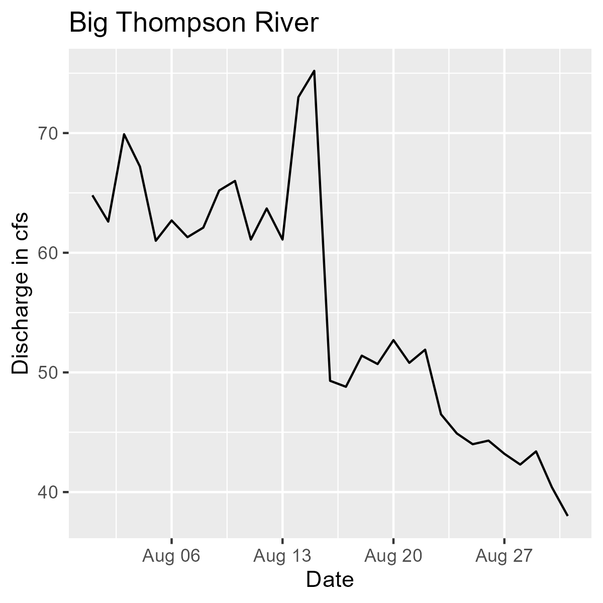
Line graph showing discharge in CFS by date for the Big Thompson River during the month of August 2018.
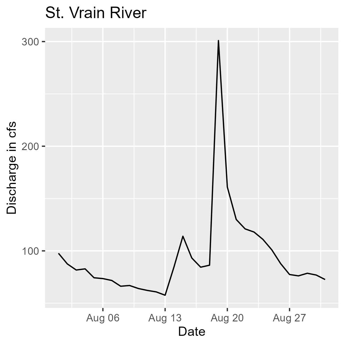
Line graph showing discharge in CFS by date for the Saint Vrain River during the month of August 2018.
We are pulling flow data for the Big Thomson River (.x[1]) and the St. Vrain River (.x[2]) for the month of August 2018. Then we are plotting each one and including the appropriate titles for the Big Thompson (.y[1]) and St. Vrain (.y[2]).
Multiple inputs: pmap()
To pass through more than 2 inputs, you must use pmap(); however, the syntax is a little different. You can pass through any number of inputs by wrapping them in a list as the first argument (.l), and they are passed to the function in the second argument (.f). If using an anonymous function, you need to make sure that it takes the same number of arguments as the length of your list (e.g., three arguments for a list with a length of 3). For example,
purrr::pmap_int(
  .l = list(
    c(1, 5, 3, 7, 5),
    c(0, 6, 7, 9, 1),
    c(4, 2, 8, 8, 6)
  ),
  .f = \(x, y, z) (x * y) + z
)
#> [1]  4 32 29 71 11
More realistically, let’s download Big Thompson and St. Vrain River data and specify a unique start and end date for each.
purrr::pmap(
  .l = list(
    site_id = c(big_tmpsn = "06741510", st_vrain = "06730525"),
    start_date = c("2018-08-01", "2019-09-01"),
    end_date = c("2018-09-30", "2019-10-15")
  ),
  .f = \(site_id, start_date, end_date) readNWISdv(
    siteNumbers = site_id,
    parameterCd = "00060",
    startDate = start_date,
    endDate = end_date
  ) |>
  tibble::as_tibble()
)

#> $big_tmpsn
#> # A tibble: 61 × 5
#>    agency_cd site_no  Date       X_00060_00003 X_00060_00003_cd
#>    <chr>     <chr>    <date>             <dbl> <chr>
#>  1 USGS      06741510 2018-08-01          64.8 A
#>  2 USGS      06741510 2018-08-02          62.6 A
#>  3 USGS      06741510 2018-08-03          69.9 A
#> # ℹ 58 more rows
#> # ℹ Use `print(n = ...)` to see more rows
#>
#> $st_vrain
#> # A tibble: 45 × 5
#>    agency_cd site_no  Date       X_00060_00003 X_00060_00003_cd
#>    <chr>     <chr>    <date>             <dbl> <chr>
#>  1 USGS      06730525 2019-09-01         104   A
#>  2 USGS      06730525 2019-09-02          99.1 A
#>  3 USGS      06730525 2019-09-03          94   A
#> # ℹ 42 more rows
One useful technique when using pmap() is to store information and data in rows of a data frame and iterate over the rows of the data frame. In this scenario we have our data stored like this.
| site_nm | site | start | end | param | param_nm |
|---|---|---|---|---|---|
| big_thompson | 06741510 | 2018-08-01 | 2018-09-30 | 00060 | flow_cfs |
| st_vrain | 06730525 | 2019-09-01 | 2019-10-15 | 00060 | flow_cfs |
| clearwater | 13341050 | 2014-07-01 | 2014-09-15 | 00010 | temp_c |
This is a great way to store data for our own reference – data in this wide format is easily understood by humans. But we can’t just send this into pmap(). Under the hood, a data frame is just a fancy list where each column is a vector. So if we tried to send this into pmap() it is going to try and iterate our function column-wise, which wouldn’t make sense: we want it to be iterated row-wise. Here is how we we could implement that.
# Create parameter data frame - using `tribble()`
param_df <- tibble::tribble(
  ~site_nm,       ~site,      ~start,       ~end,         ~param,  ~param_nm,
  "big_thompson", "06741510", "2018-08-01", "2018-09-30", "00060", "flow_cfs",
  "st_vrain",     "06730525", "2019-09-01", "2019-10-15", "00060", "flow_cfs",
  "clearwater",   "13341050", "2014-07-01", "2014-09-15", "00010", "temp_c"
)

# Mapping over rows of `param_df` download data using parameters
purrr::pmap(
  .l = param_df,
  .f = \(...) {
    params <- tibble::tibble(...)
    dataRetrieval::readNWISdv(
      siteNumbers = params$site,
      parameterCd = params$param,
      startDate = params$start,
      endDate = params$end
    )
  }
)
Why does this work. Let’s remove the readNWISdv() part of the code above and just have it return the data frame (or tibble in this case) that is passed through for each iteration.
purrr::pmap(
  .l = param_df,
  .f = \(...) tibble::tibble(...)
)

#> [[1]]
#> # A tibble: 1 × 6
#>   site_nm      site     start      end        param param_nm
#>   <chr>        <chr>    <chr>      <chr>      <chr> <chr>
#> 1 big_thompson 06741510 2018-08-01 2018-09-30 00060 flow_cfs
#>
#> [[2]]
#> # A tibble: 1 × 6
#>   site_nm  site     start      end        param param_nm
#>   <chr>    <chr>    <chr>      <chr>      <chr> <chr>
#> 1 st_vrain 06730525 2019-09-01 2019-10-15 00060 flow_cfs
#>
#> [[3]]
#> # A tibble: 1 × 6
#>   site_nm    site     start      end        param param_nm
#>   <chr>      <chr>    <chr>      <chr>      <chr> <chr>
#> 1 clearwater 13341050 2014-07-01 2014-09-15 00010 temp_c
By sending our data through this way, we are now forcing pmap() to see the data as a list of rows rather than a list of columns. This, of course violates the style principle mentioned earlier that data functions should be named and not anonymous if they require { }. We tend to see this as an exception because we use the tibble::tibble(...) line to clue us into how the function is working (i.e., row-wise).
For more information on mapping with multiple inputs, see 10 Map with multiple inputs | Functional programming .
No outputs: walk()
walk() works similarly to map(), but is used for cases where a side effect is desired. Instead of returning the output of the function in a list (like map()), it returns the input. This allows a side effect to be performed in the middle of a pipe chain.
list(c(TRUE, FALSE, TRUE), c(1, 5, 3, 6, 4)) |>
  purrr::walk(.f = print) |> # .x is being piped in from the line above
  purrr::map_dbl(sum)
#> [1]  TRUE FALSE  TRUE
#> [1] 1 5 3 6 4
#> [1]  2 19
In this example, the list is printed, which explains the first two lines of console output, and then each vector is summed and returned as a numeric vector, which is the last line (two TRUEs = 2, and 1 + 5 + 3 + 6 + 4 = 19).
One of the most common use cases for walk() or its variant walk2() is to write files to disk.
tempdir <- tempdir()

purrr::walk2(
  .x = list(mtcars, iris),
  .y = file.path(tempdir, c("mtcars.csv", "iris.csv")),
  .f = \(df, path) readr::write_csv(df, file = path)
)
This will iterate pairwise the two input lists (or in this case list and vector) to write each data frame from the first list to the path specified in the second list (or vector). For just two data frames this might not save you much time or effort, but if you are writing many, it has to potential to save you a headache.
For more information on using walk(), see No outputs: walk() and friends | Advanced R
.
Closing thoughts
Incorporating the purrr::map_*() family of functions into your R code can rapidly accelerate the efficiency, accuracy, and readability of your code. With it, we can do away with copy-and-paste programming
and continue our journey to writing more transparent, accurate, and effective code.
References and further reading
- Lists and vectors
- Purrr and mapping
Categories:
Related Posts
Reproducible Data Science in R: Flexible functions using tidy evaluation
December 17, 2024

Overview
This blog post is part of a series that works up from functional programming foundations through the use of the targets R package to create efficient, reproducible data workflows.
Reproducible Data Science in R: Writing better functions
June 17, 2024
Overview
This blog post is part of a series that works up from functional programming foundations through the use of the targets R package to create efficient, reproducible data workflows.
Reproducible Data Science in R: Writing functions that work for you
May 14, 2024
Overview
This blog post is part of a series that works up from functional programming foundations through the use of the targets R package to create efficient, reproducible data workflows.
Reproducible Data Science in R: Say the quiet part out loud with assertion tests
September 2, 2025

Overview
This blog post is part of the Reprodicuble data science in R series that works up from functional programming foundations through the use of the targets R package to create efficient, reproducible data workflows.
A map that glows with the vocabulary of water
February 27, 2026
English is the official language and authoritative version of all federal information.
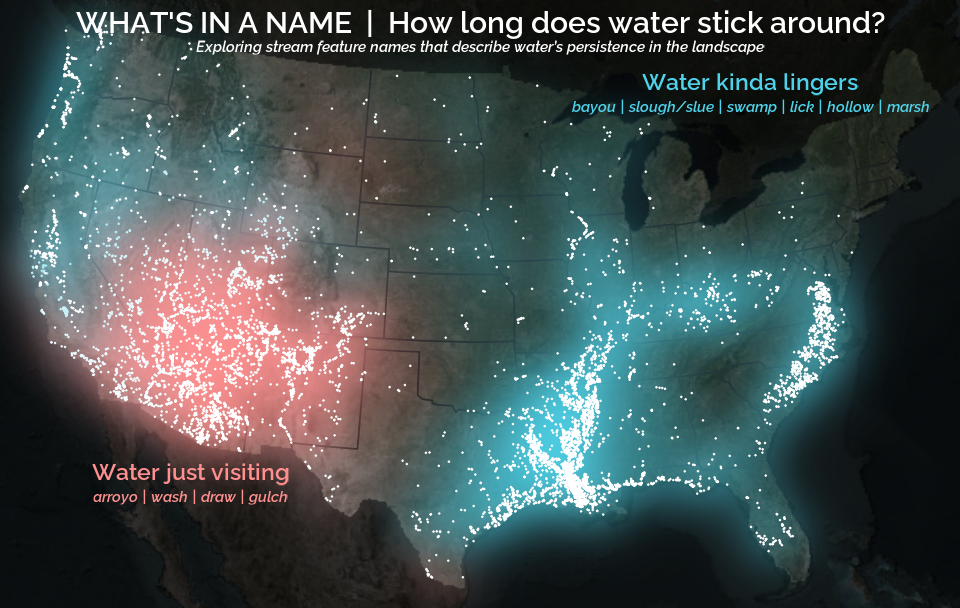
A map that glows with the vocabulary of water
What is your first impression of the map above? To me, it is the shimmer. Thousands of points of light, each one a stream or river, illuminating a darkened basemap. Look closely and a pattern emerges: the country’s waterways form a linguistic constellation. These points are classified not from population data or even explicitly by hydrology. They glow strictly according to the vocabulary used to name them and what can be implied about the hydrology of these streams based on their names.